Haneskjellfeltene ved Moffen og Parryflaket, nord av Svalbard, ble kartlagt i august 2022. Toktet var den første dedikerte undersøkelsen av disse skjellfeltene siden haneskjellfisket ble stengt for 30 år siden, etter flere år med et overfiske som ødela bestanden. Transekter med undervanns video ble gjennomført innenfor og utenfor verneområdet, og skrapestasjoner ble tatt parallelt med videotransektene utenfor verneområdet. Skraping ble benyttet for å samle biologiske prøver, både til å bestemme størrelses- og alderssammensetning, til vevsanalyser på fremmed- og næringsstoffer, og til populasjonsgenetiske analyser. Parallelle video- og skrapestasjoner ble dessuten brukt til å sammenligne tetthetene av haneskjell mellom de to redskapstypene. Stillbilder ble tatt fra videoopptakene og brukt til haneskjellannotering. Annoteringen av skjell fra stillbildene fra hver stasjon, ble gjenomført av flere personer uavhengig av hverandre, for å analysere usikkerheten i skjelltellingen. Resultatene fra toktet viste at bestandene på begge haneskjellfeltene var på samme nivå eller høyere enn det som ble observert på feltene ved Bjørnøya i 2019 og 2020. Bestandsstørrelse ved Moffen og på Parryflaket ble estimert til å være høyere enn på de tre Bjørnøya-feltene til sammen, mens skjellstørrelsen og dermed andelen over minstemålet var mindre. Geostatistiske modeller til bestandestimering ble testet, og det viste seg at slike romlige modeller kan håndtere den betydelige romlige variasjonen i bestandstetthet bedre enn tidligere design-baserte metoder. I tillegg kan en modell-basert tilnærming brukes til å inkludere habitat- og miljøvariabler for å forklare variasjonen i skjelltetthet, til å estimere usikkerhet i estimatene, og for å kombinere video- og skrapeobservasjoner i et felles estimat. Dette øker oppløsingen i datasettet, og kan gjøre mulig å sammenligne med tidligere undersøkelser med skrape. Basert på resultatene anbefaler vi å inkludere haneskjellfeltene ved Moffen og på Parryflaket i det pågående prøvefisket for å fordele fiskeinnsatsen på flere skjellfelt og dermed på en større bestand.
Survey of Iceland scallop beds north of Svalbard
— Survey number 2022839
Report series:
Toktrapport 2023-17
ISSN: 1503-6294
Published: 11.01.2024
Cruise no.: 2022839
Research group(s):
Bentiske ressurser og prosesser
Subject:
Haneskjell
Program:
Barentshavet og Polhavet
Approved by:
Research Director(s):
Geir Huse
Program leader(s):
Maria Fossheim
Norsk sammendrag
Summary
In August 2022, the scallop beds of Moffen and Parryflaket north of Svalbard were surveyed to assess the state and distribution of Iceland scallops (Chlamys islandica). This represented the first investigation in 30 years after the closing of the scallop fishery in the area, following several years of destructive overfishing. The survey was conducted with video transects inside and outside the protected areas, and dredge stations outside the protected areas parallel to video transects. Dredging was used to collect biological samples for size and age composition, and tissue samples for contaminant, nutrient and population genetic analysis. Furthermore, parallel stations allowed to compare observed scallop densities between dredge and video. Still images were extracted from video to annotate scallops, with repeated annotations of all stations by multiple persons. The results show that the stocks on both scallops bed have recovered from previous fishing to densities that are comparable or higher than those observed in the Bear Island area. The scallop abundance at the two scallop beds combined is estimated to be higher than on the three Bear Island scallop beds, whereas the scallops on Moffen and Parryflaket tended to be smaller and therefore the proportion above minimum legal landing size lower. Geostatistical approaches were tested to estimate density and abundance. Compared to previous design-based approaches, spatial modelling captures the spatial variation in density more adequately, allows for including links to habitat and environment, and to estimate uncertainty of estimates. Furthermore, video and dredge data could be integrated into a joint estimate, improving the resolution and historic comparability. We recommend to consider the inclusion the scallop beds north of Svalbard into the trial fishery to spread fishing effort across a larger stock and area.
Background and objectives
The goal of the IMR cruise 2022839 was to survey north of Svalbard areas near Moffen and on the Parryflaket where beds of Iceland scallops (Chlamys islandica) are known to occur based on survey and fisheries data from the late 1980ies. Moffen was a key area in the former fishery for Iceland scallops. A relevant part of the scallop distribution observed on two surveys in 1986 and 1988 are today within the Svalbard protection zone and therefore not accessible for exploitation. However, relevant areas are outside of protected zones and could sustain a fishery if the stock has rebuilt after past overexploitation. Similar surveys in 2019 and 2020 showed that scallop beds around Bjørnøya and on Spitsbergenbanken have largely recovered, and a trial fishery starting in 2022 has been allowed in those areas with an annual TAC of 15,000 tonnes. The Moffen area may increase the possible sustainable catches substantially given sufficient shell density in the zone outside of the protected areas.The specific aim of cruise no 2022839 were as follows:
1. Map the distribution and density of Iceland scallops in the Moffen and Parryflaket areas using video transects and dredge stations.
2. Estimate total abundance in the areas based on density information and potential explanatory variables such as bottom depth.
3. Compare shell counts from parallel dredge and video stations to estimate catchability coefficients and evaluate the inclusion of dredge catches for abundance estimation.
4. Gather representative biological data to create size frequency distributions and age-size keys, as well as collect tissue samples for population genetic analyses, contaminant and nutrient analysis.
5. Investigate the spread of snow crab in inshore areas north(-west) of Svalbard and potentially into Hinlopen straight.
Methods
Survey plan and design
Area polygons were created based on survey data from 1986 and 1988, enclosing the areas north of Moffen and on Parryflaket where Iceland scallops were previously observed. The areas were split into substrata along the border of the Svalbard nature reserve, creating substrata based on their placement inside or outside of the protected zone. Stations were randomly drawn along a nonaligned grid and matched with bottom depth information based on the nearest available position where bottom depth is known (based on observed depth in 1986/88 and GEBCO bathymetric data). The station grid was subsequently filtered for suitable bottom depths, excluding all initial stations at bottom depths above 20m or below 150m where occurrence of Iceland scallops is highly unlikely. Positions inside the protected areas were downweighted to a 1/10 probability compared to those outside to ensure a majority of stations outside of protected areas. Similarly, the probability for stations in the Moffen area following the eastern border of the protection zone was down weighted due to suboptimal bottom substrate.
The remaining stations were randomly reduced to a total of 84 stations, with half of them defined as backup stations. The number of main stations (42) was determined based on bootstrapping analysis of survey data from the Bjørnøya and Spitsbergenbanken areas in 2019 and 2020 that was used to determine the ratio of stations per area that generates a stable mean density estimate. Of the main stations outside of the protected areas, 15 were randomly selected as combined dredge and video stations, in contrast to the rest where only video transects were conducted. Furthermore, four stations for snow crab traps were placed manually at locations of interest within fjords of northwestern Spitsbergen island.
Sampling procedure
Video transect
At video stations, a metal frame sledge equipped with a video camera, lights and lasers was towed along the seafloor (Figure 1). A GoPro Hero6 camera was mounted on a video sledge at a 90° angle, providing a horizontal view down to the sea floor. The sledge was towed for 20 minutes after bottom contact at preferable 0.5 knots. After hauling the sledge on board, video recordings were extracted, backed up, and checked to ensure that 1) the camera has worked as intended and 2) evaluate recordings regarding light conditions and vessel speed to make adjustments if needed. A temperature logger on the video sledge recorded temperature continuously while deployed.
Biological sampling
A delta dredge (Figure 1) was used to collect biological samples. The dredge was towed for 5 minutes after bottom contact, as the collection bag can fill up very quickly. Dredge catches were sorted on deck and all live scallops sorted out. All scallops were measured individually using electronic bluetooth calipers (shell height). The first 10 scallop samples were retained for ageing, population genetics, contaminants and nutrient analysis: scallops were opened to remove 1) muscle tissue, 2) gonads and 3) digestive glands (hepatopancreas) with a scalpel and freeze them separately in plastic tubes; subsequently, tissue from the gills was removed and stored in plastic tubes with alcohol; lastly, the shells were cleaned and frozen for ageing on land.
Ageing procedure
The clean shells of scallops were thawed in freshwater for 5-10 minutes before the two shells were seperated by cutting the ligament with a scalpel. Then we removed the soft parts of the ligament carefully with a scalpel, using a stereo magnifier. We kept the ligament wet during the process, using the hard part of the ligament for age determination. The hard ligament is pyramid shaped, and new layers and light and dark zones are deposited as the shell grows. A drop of freshwater was put on the hard ligament, and the number of zones were counted. The first year’s growth line is often difficult to see, and this must be taken into account when determining age. Age reading usually starts from the 2nd year’s growth line.
Contaminant and nutrient analysis
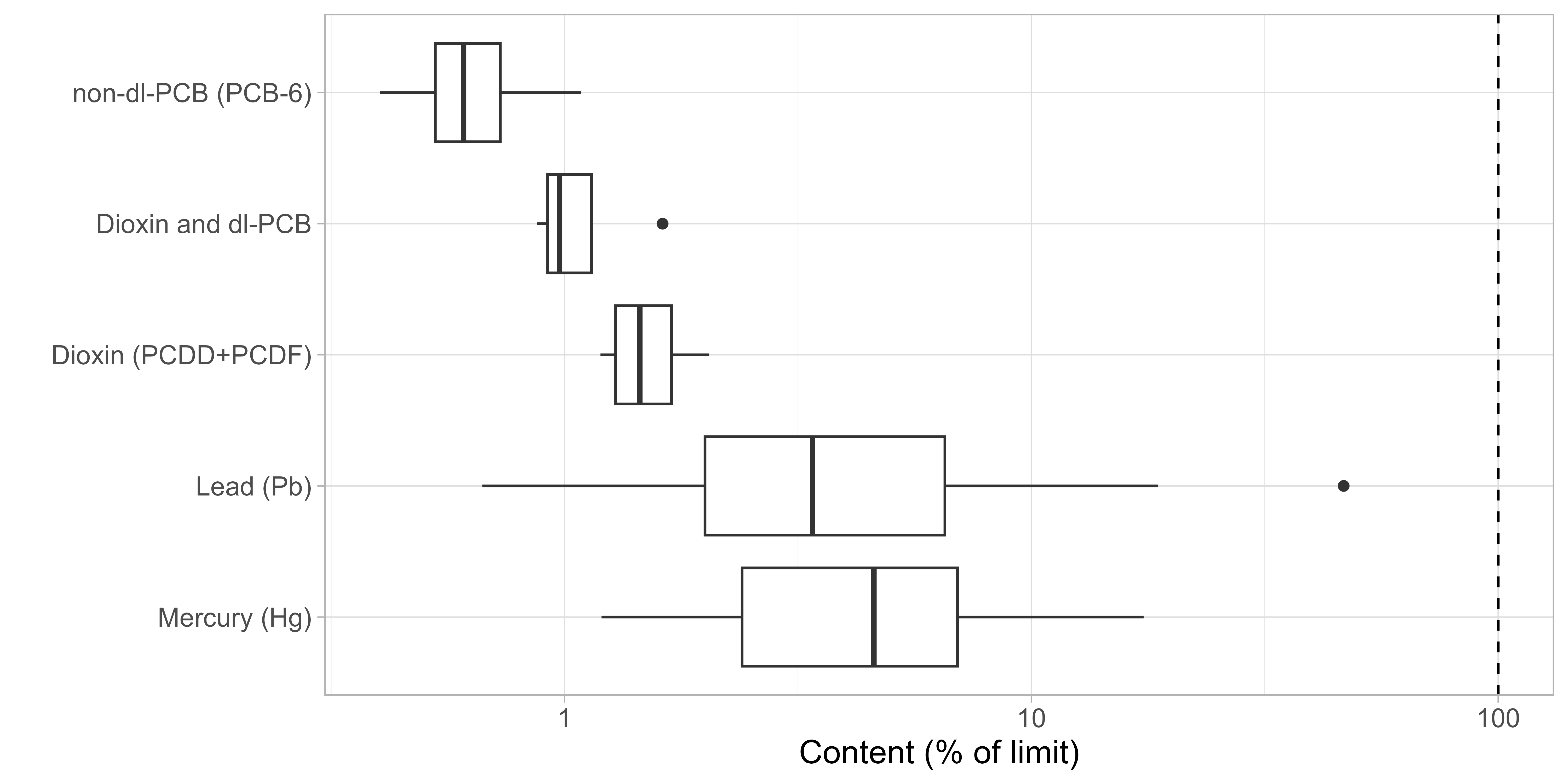
Samples of muscle, hepatopancreas and gonad taken from individual scallops from dredge stations were analyzed for metals. In addition, composite samples of muscle, hepatopancreas and gonad were prepared and analyzed for persistent organic pollutants including the sums of dioxins and furans (PCDD/F), PCDD/F and dioxin-like PCBs (PCDD/F+dlPCB), and the EU selected non-dioxin like-PCBs (PCB6). The composite samples of hepatopancreas and gonad were also analyzed for metals. The applied analytical methods are listed in Zhu et al (2023). The results were compared with existing maximum levels for the scallop Pecten maximus foodstuffs given in EU regulation 1881/20062023/915 and the Norwegian regulation FOR-2015-07-03-870, due to its anatomical similarity. The maximum levels for metals apply to the adductor muscle and gonad only, while for dioxins and PCBs all soft tissues are considered.
Snow crab expansion
Four strings with five conical snow crab pots (Figure 1) each were deployed at selected locations in the deep basins of Raudfjorden, Woodfjorden and Wijdefjorden. The pots were baited with herring and caught individuals were identified on board. Temperature loggers were fixed on the snow crab pots to register temperature during the entire soaktime.
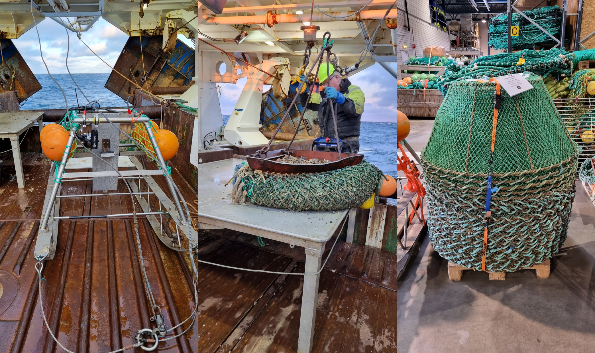
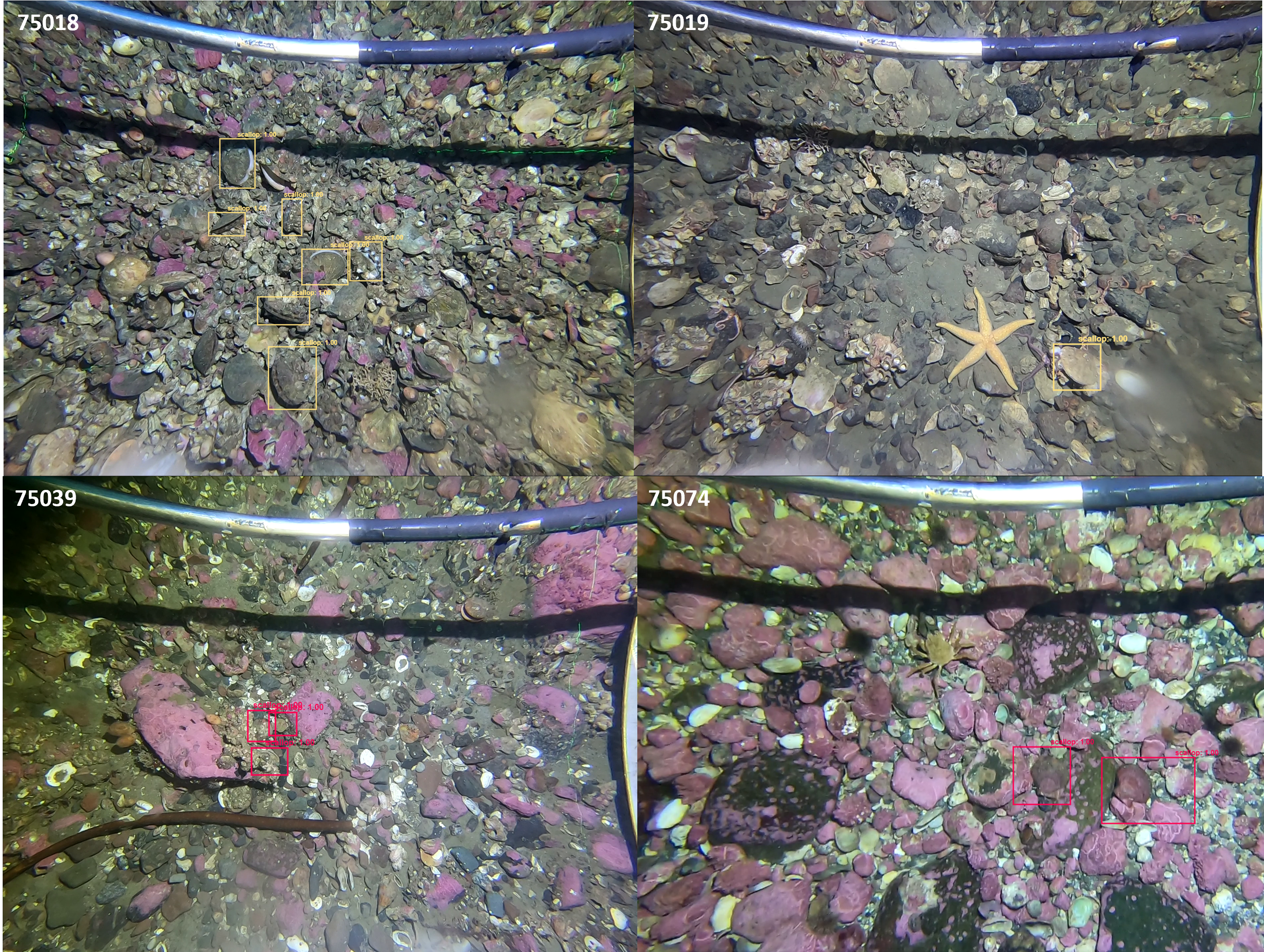
Image annotation
Preliminary analysis of video transects showed that quality of video images was insufficient to reliably identify live scallops along the entire transect. The main reasons were speed and visibility that make it difficult or impossible to clearly determine organism on the sea floor. For all video transects, still images were extracted for all sequences where image quality was considered sufficient for annotation and counting of scallops. The approach resulted in average in 55.95 per station (minimum 3, maximum 135).Scallops on still images of each station were annotated by multiple people, ensuring at the minimum duplicated counts of scallops per station. The aim was to use repeated countings to validate counts and estimate counter variation and potential bias. Scallops were annotated by five people independently, with varying experience with Iceland scallops, benthic organisms and image annotation. Images were processed and annotated in DIVE (https://kitware.github.io/dive/). For further details see Stokkeland (2023).
Additional data
For comparison, data on scallop densities and stock composition from IMR’s Iceland scallop surveys in 2019 and 2020 in the Bear Island area were used. For further information see Sundet and Zimmermann (2020) and Stokkeland (2022).
Physical ocean data from the TOPAZ4 Arctic Ocean system (https://doi.org/10.48670/moi-00001) were included to provide information on current velocity and direction, mixed-layer depth, salinity and temperature. For descriptions of the underlying ocean model see Melsom et al. (2012) and Sakov et al. (2012). Monthly averages were extracted from the ocean model grid and matched with the closest survey observations to evaluate them as potential covariates explaining variation in scallop density.
Statistical analysis and stock estimation
Densities per station were estimated from annotated scallop counts per image across all counters and images using a generalized mixed effect model (GLMM) with scallop count as response, assuming a negative binomal error distribution. Counters were included as random intercept. The GLMM was implemented in glmmTMB. The estimated means per station were used either as observed density or together with estimated standard errors as a probability distribution. The latter was done to explore how counting uncertainty affects stock estimates.
To facilitate comparability of dredge and video as well as between the video sledge used in 2022 and 2020 with the video rig used in 2019, all scallop counts were standardized to m2. As observed areas, the image frame determined by lasers (0.495 m2 and 0.423 m2 in 2020/22 and 2019, respectively) were used for video images and a swept width of 0.5 m multiplied with towing distance for dredge stations.
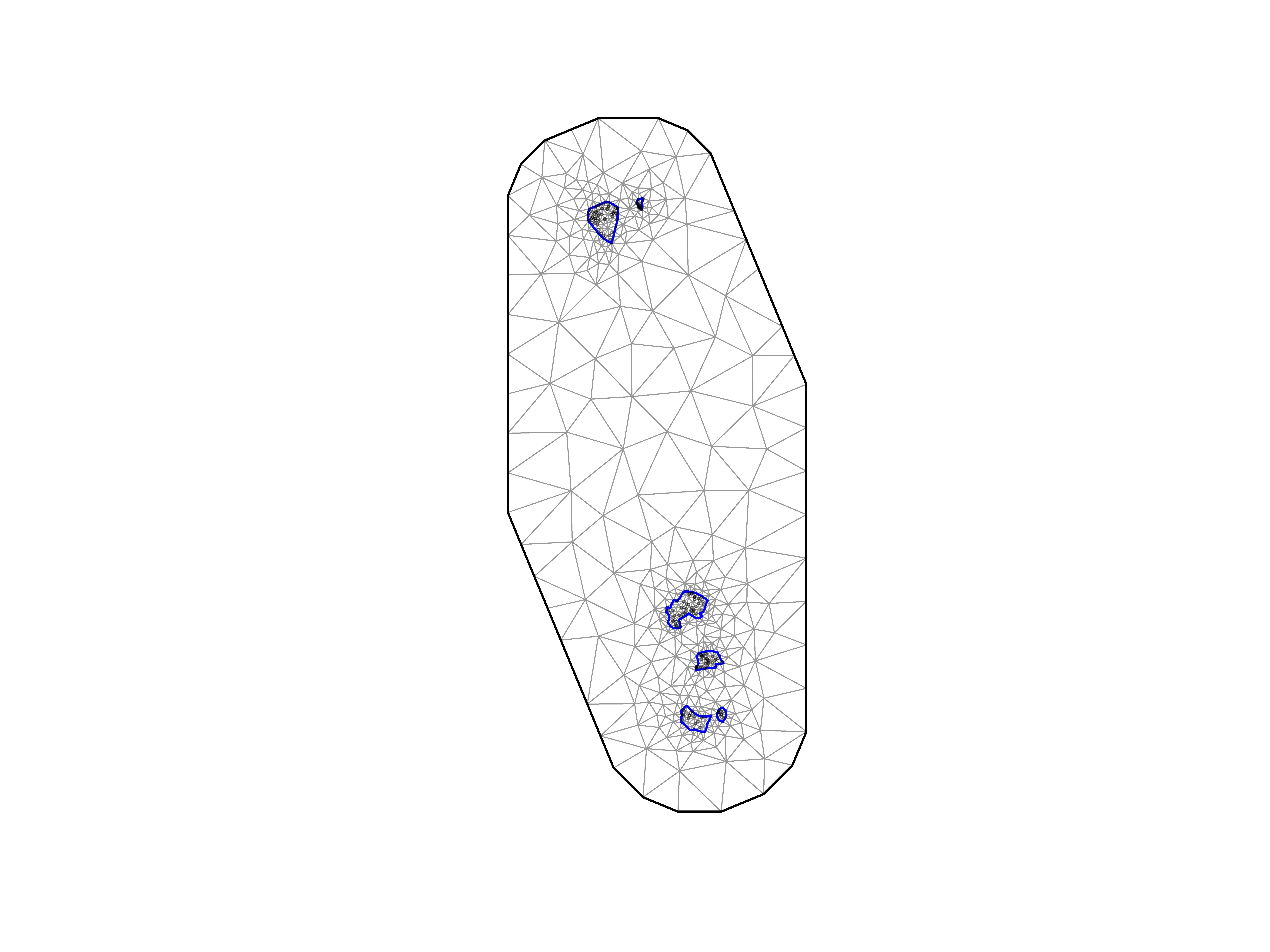
Density was modeled as number of scallops per m2 with a spatial generalized additive model (GAMM) with spatial Gaussian Markov random fields implemented in sdmTMB (Anderson et al 2022, https://pbs-assess.github.io/sdmTMB/index.html). The response variable was assumed to follow a compound Poisson-gamma tweedie distribution with log-link: Tweedie( μ ,p, φ ) where 1< p <2. Explanatory variables were included as categorical fixed effects for stratum (scallop) bed and gear type (video rig (used in 2019), video sledge (2020 and 2022), dredge), and as continuous fixed effects for bottom depth and environmental variables with thin plate regression splines restricted to 3 degrees of freedom. The mesh for the spatial random field was created with refined Delaunay triangulation (Bakka et al 2018) constrained to the scallop bed boundaries with maximum edge length of 8 km inside of the boundaries, 100 km outside, a cutoff distance of 2 km, and a minimum triangle angle of 25°. Model configuration and backward model selection was conducted using AIC sensu Zimmermann et al (2023). The integration grid for spatial predictions was created as a regular grid with a grid cell area of 0.4 km2, using the nearest GEBCO bathymetric information (https://www.gebco.net/) for each integration point as bottom depth, TOPAZ4 Arctic Ocean system data for environmental information, and setting the gear effect to video.
After model selection, four specific model configurations were tested: 1) integrating density data from video and dredge as response variable; 2) as in 1) but weighted by the number of images per station (
Length and age frequency distributions were estimated using the spatial GAMM approach developed by Breivik et al (2021). The approach was recently integrated with a spatial model to estimate age-length keys (Breivik et al in prep.). Here we used the integrated length-age implementation (https://github.com/NorskRegnesentral/spatioTemporalIndices) to estimate number at length, age-length key, and number at age.
Results
Station overview
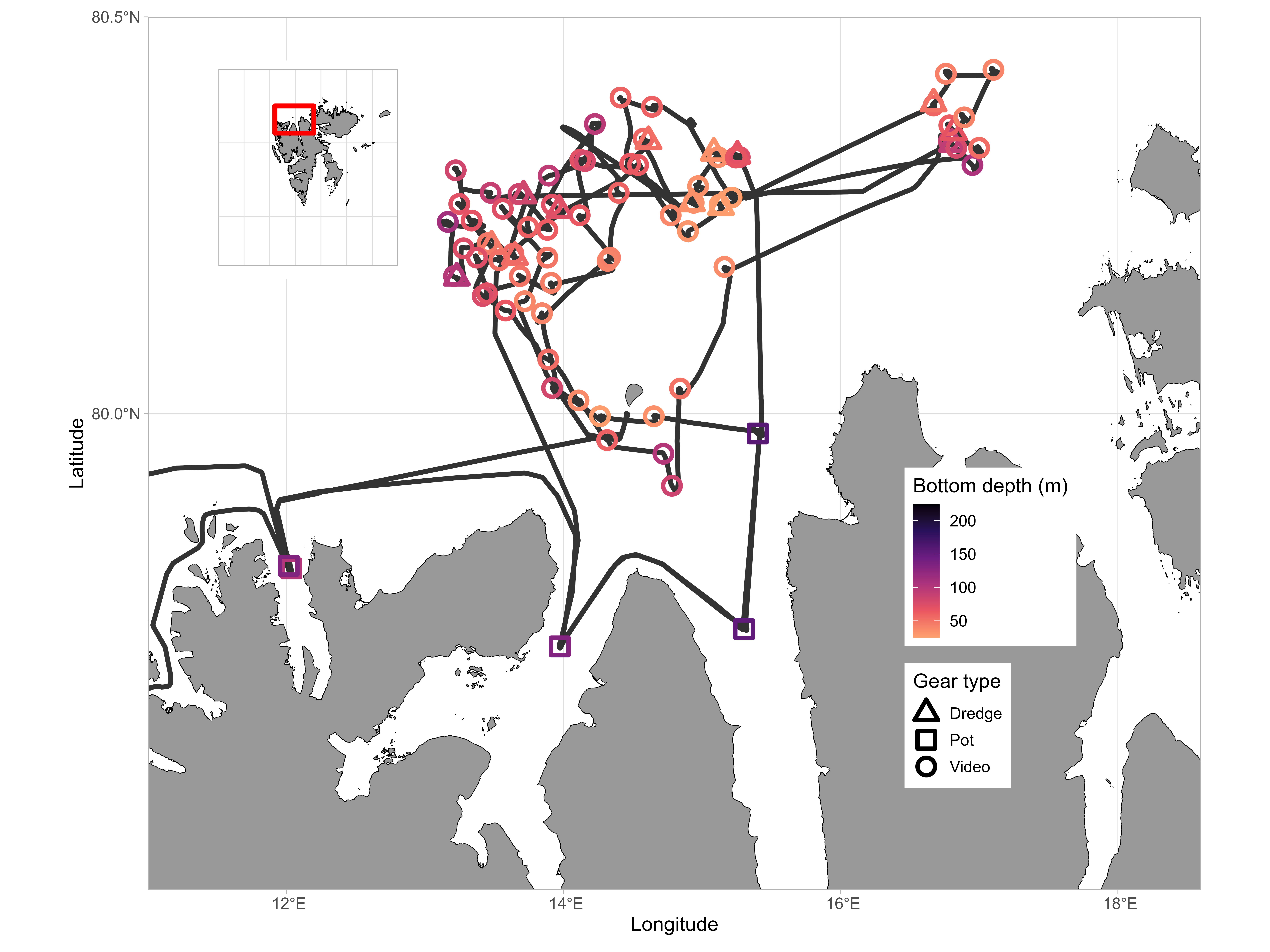
In total, the survey covered between 20-25th of September 2023 the Moffen and Parryflaket scallop beds with 66 video transects and 13 dredge stations. In addition, snow crab pots were set at four stations. Mean bottom depth of dredge and video stations was 61m (range 25 - 111m). A complete station list is shown in the Annex (Table 3).
Scallop densities
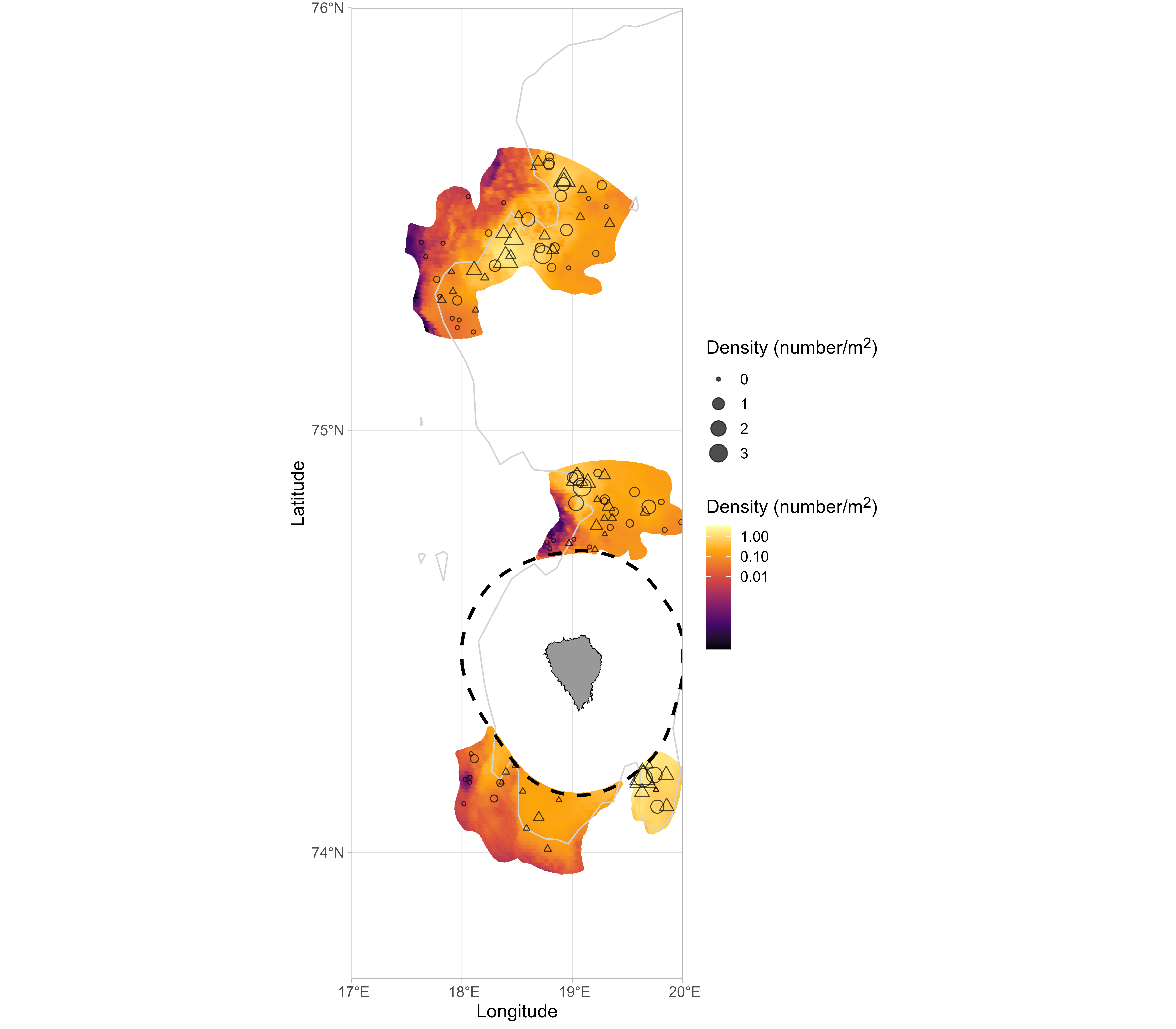
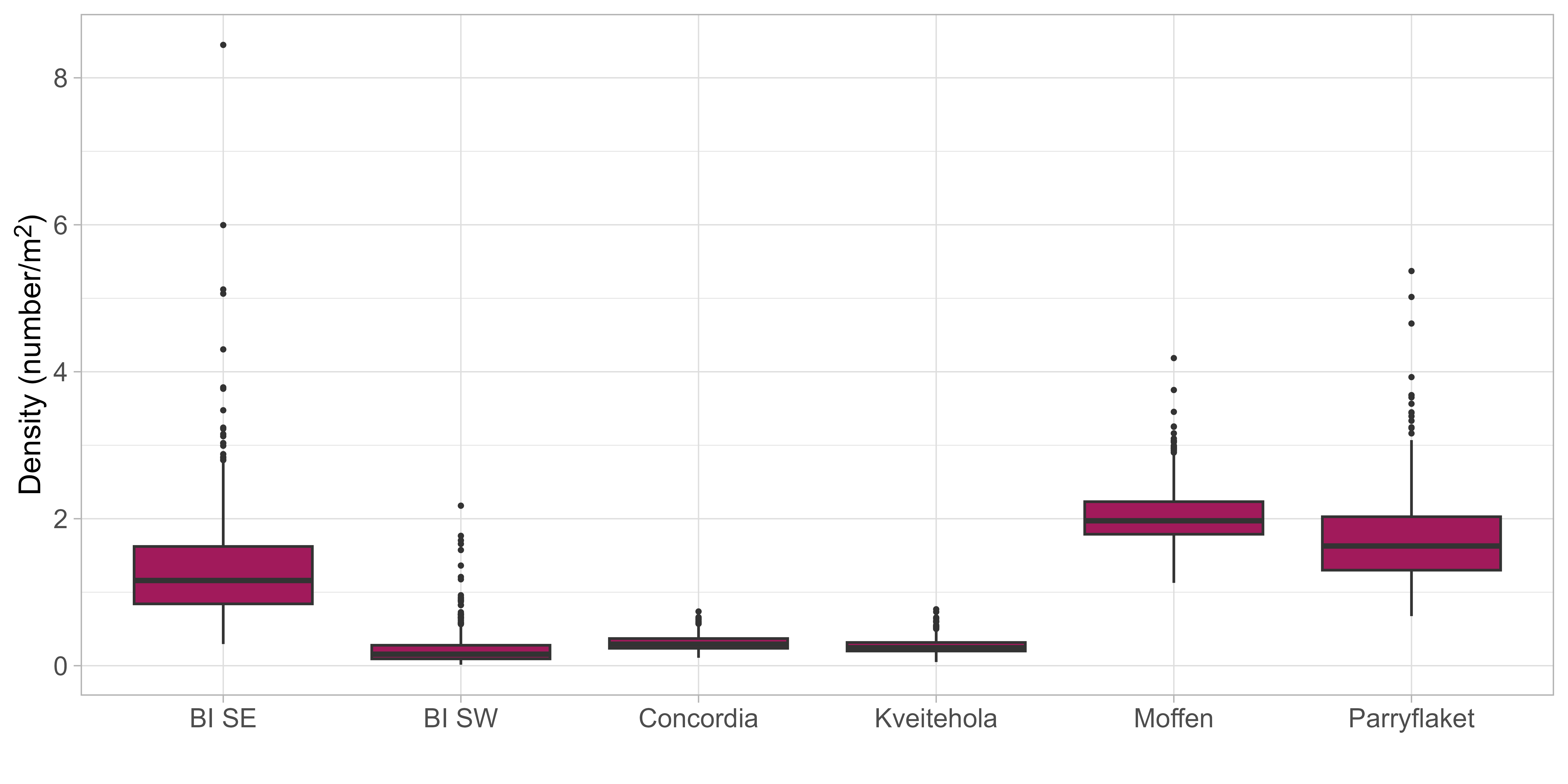
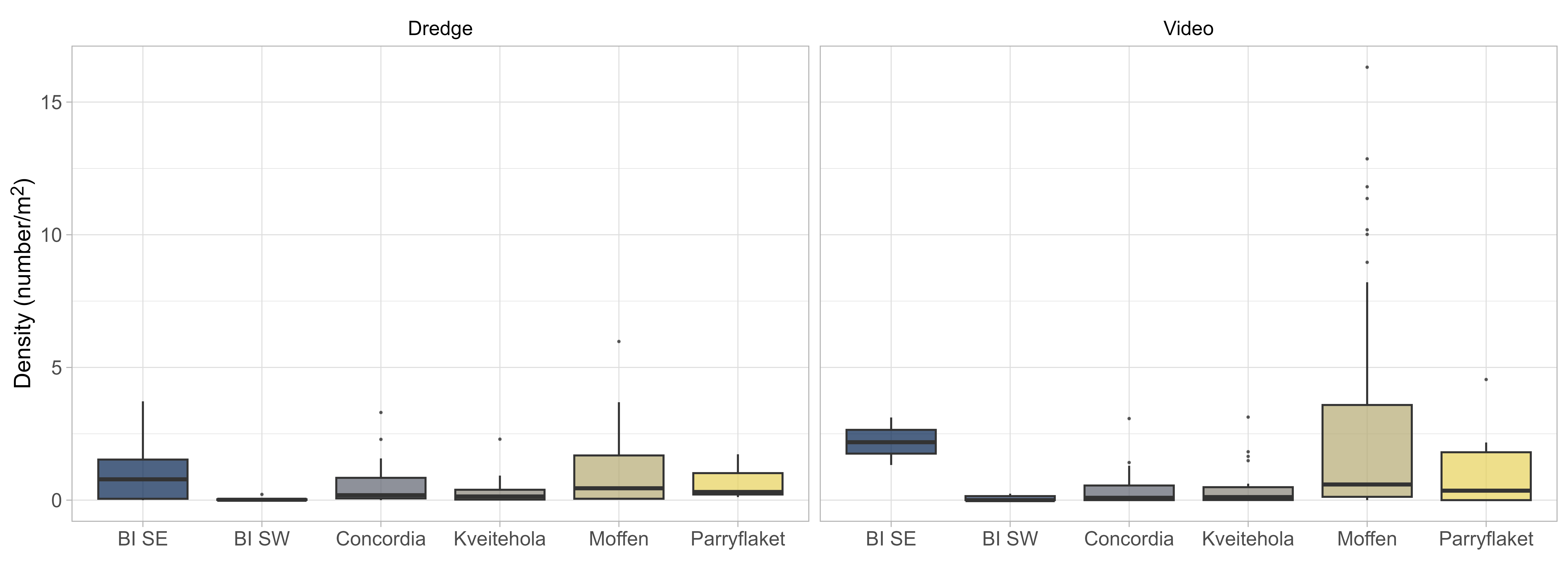
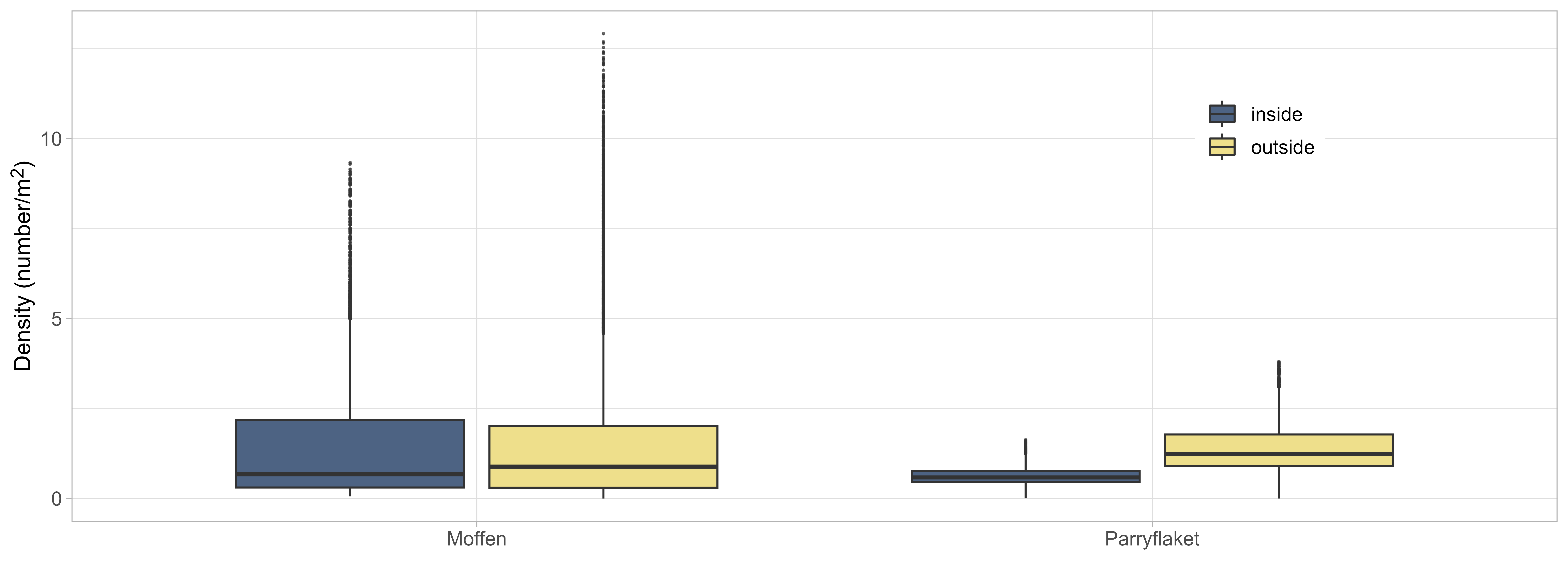
Scallop presence in the surveyed area was high, with scallops entirely absent on only 4 out of 73 stations. Scallop distribution was, however, found to be very patchy, and there was large variation between stations regarding registered scallop counts. Observed number of scallops ranged from 1 to 1090 per station, corresponding to densities between 0.005 and 16.313 scallops per m2 . Scallop densities on Moffen and Parryflaket beds were high compared to those observed in the Bear Island area in 2019 and 2020 (Figure 4), with observed densities on Moffen and Parryflaket on a similar level as the Bear Island (Southeast) scallop bed.
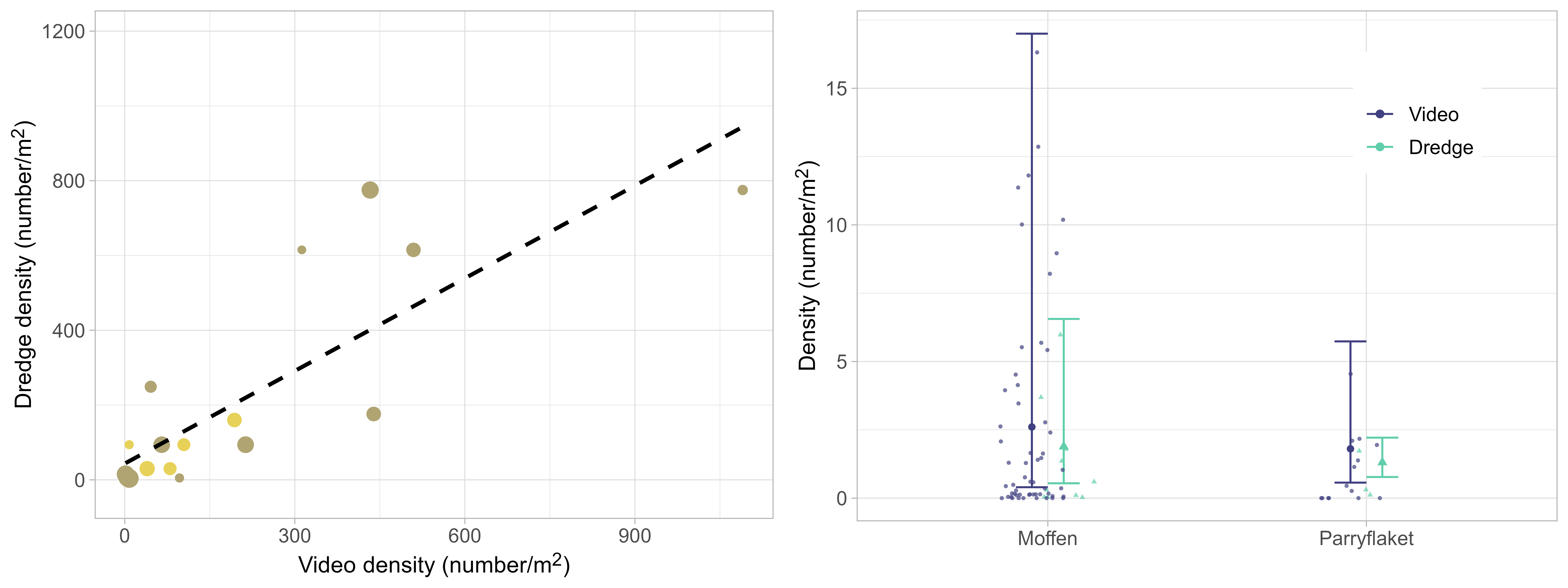
Trends in observed densities were consistent between video transect and dredge stations, with a clear correlation between counted scallops on parallel stations (Figure 5, left). This allowed for integrating data from both gear types in the GAMM used to estimate density and abundance, including gear as a categorical effect. The parameter estimates showed a tendency for lower densities at dredge stations, but the effect was minor and not significant (Figure 5, right).
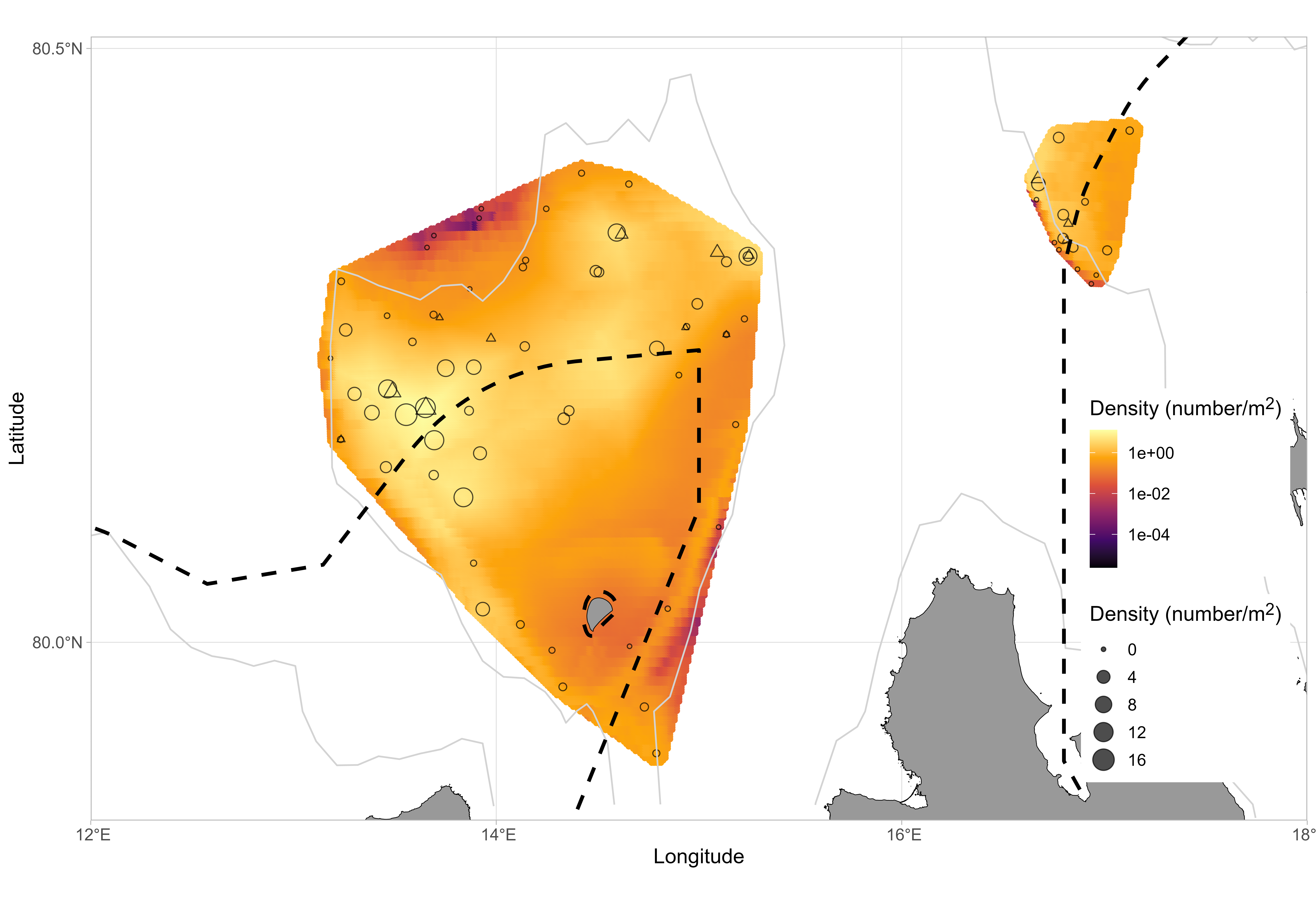
Estimated density distribution showed scallop hotspots on Moffen whereas densities were more evenly distributed on Parryflaket (Figure 6). Very high densities were found on northwestern Moffen bed around the boundary of the protected area, and to a lower degree northeastern areas. Densities were the lowest on the northern and southeastern limit of the surveyed area as well as around Moffen island. Differences in distribution can therefore be linked to unsuitable bottom substrate and bottom depth in those areas. On Parryflaket, less contrast was found based on fewer stations and a smaller area. Some boundary effects, i.e. relatively high densities close to the stratum boundaries, were found on both scallop beds, indicating that the extent of the distribution has not been fully covered.
Densities were similar inside and outside of the protected area on Moffen, compared to higher densities outside on Parryflaket (Figure 7). The differences can be attributed to the border line of the protected area that splits relevant scallop habitats on Moffen evenly, while on Parryflaket the protected area tends to be shallower and less suitable.
Relationship with bathymetry and environment
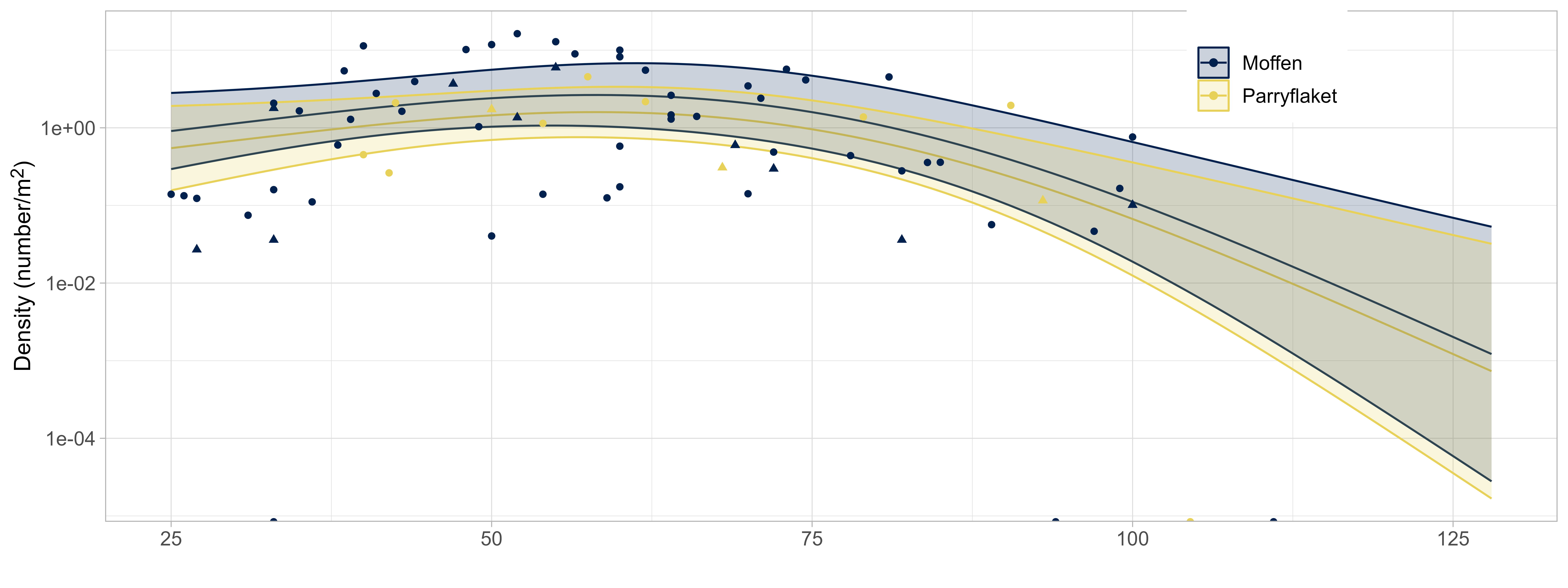
Stock density was estimated using spatial GAMMs. The selected model configuration based on AIC included bottom depth as a spline, in addition to stratum (scallop bed) and gear type as categorical variables (see Annex). The relationship with bottom depth was estimated as a concave curve with increased scallop density at intermediate depth, peaking around 70m (Figure 8. Due to the large variation in observed scallops across the entire depth range, the depth effect is relatively minor and uncertain. However, there is a clear trend towards consistently low densities at very shallow (<30m) or deep bottom depth (>100), confirming prior results from the Bear Island area (Sundet & Zimmermann 2020).
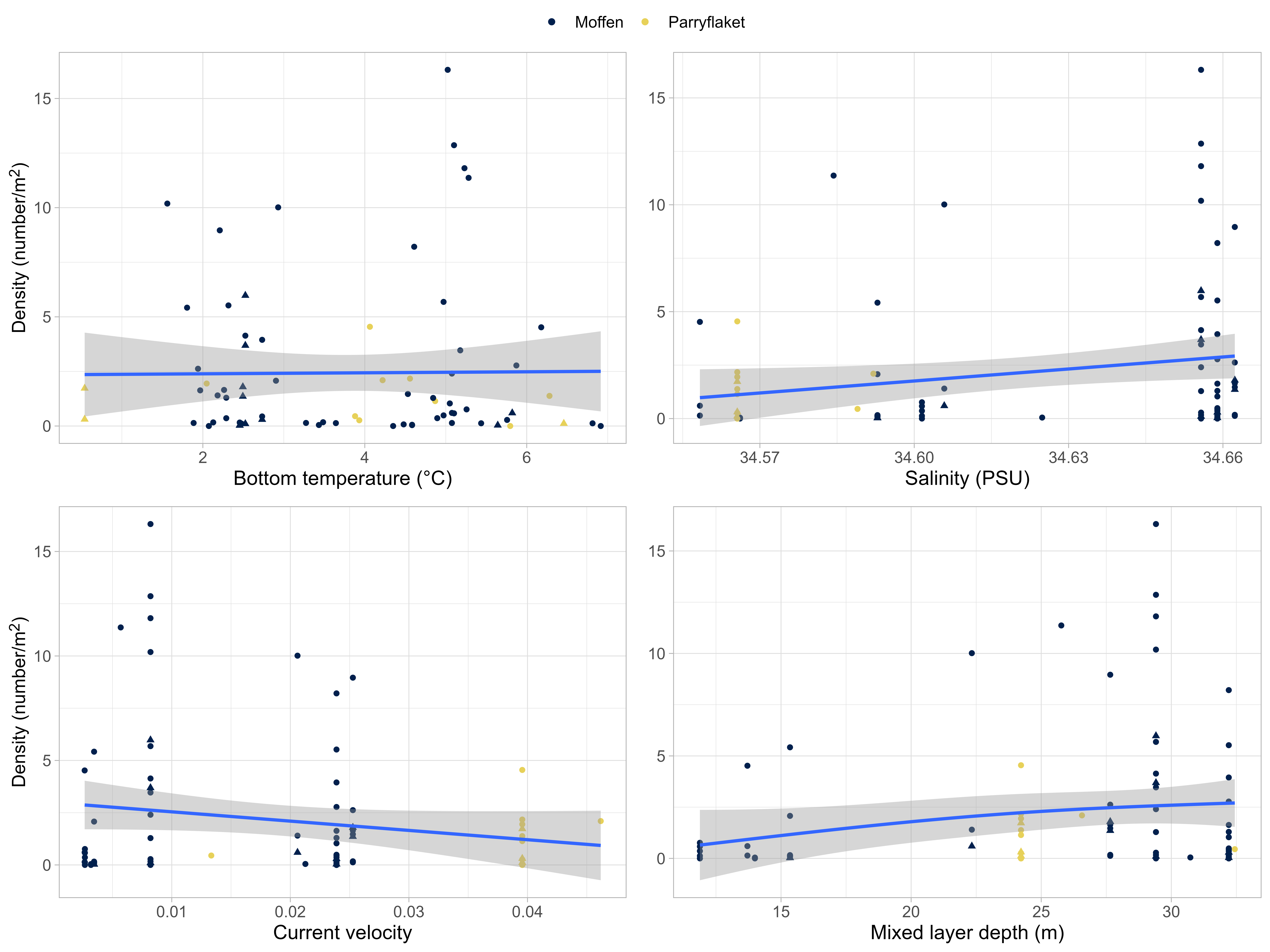
Links between scallop density and other environmental variables were explored. Although there were some indications of trends, specifically for salinity, current velocity and mixed layer depth (Figure 9, the effects were found to be not relevant during model selection (9.3). Preliminary analysis was also conducted using information on bottom substrate (grain size). Bottom substrate can be considered as a key predictor of scallop abundance, but the comparatively coarse resolution of the data did not provide sufficient contrast to explore its role further.
Intra-transect variation and uncertainty
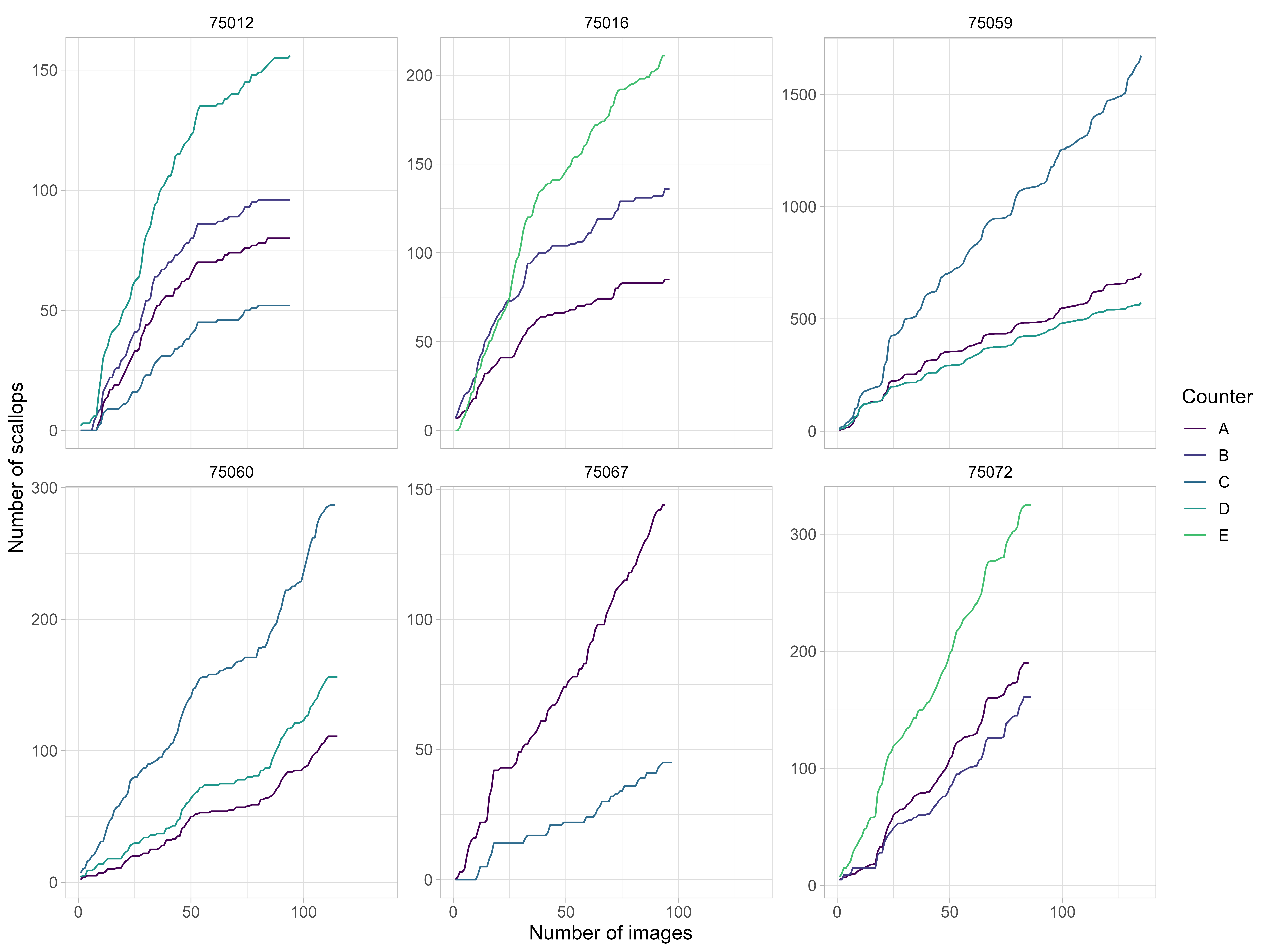
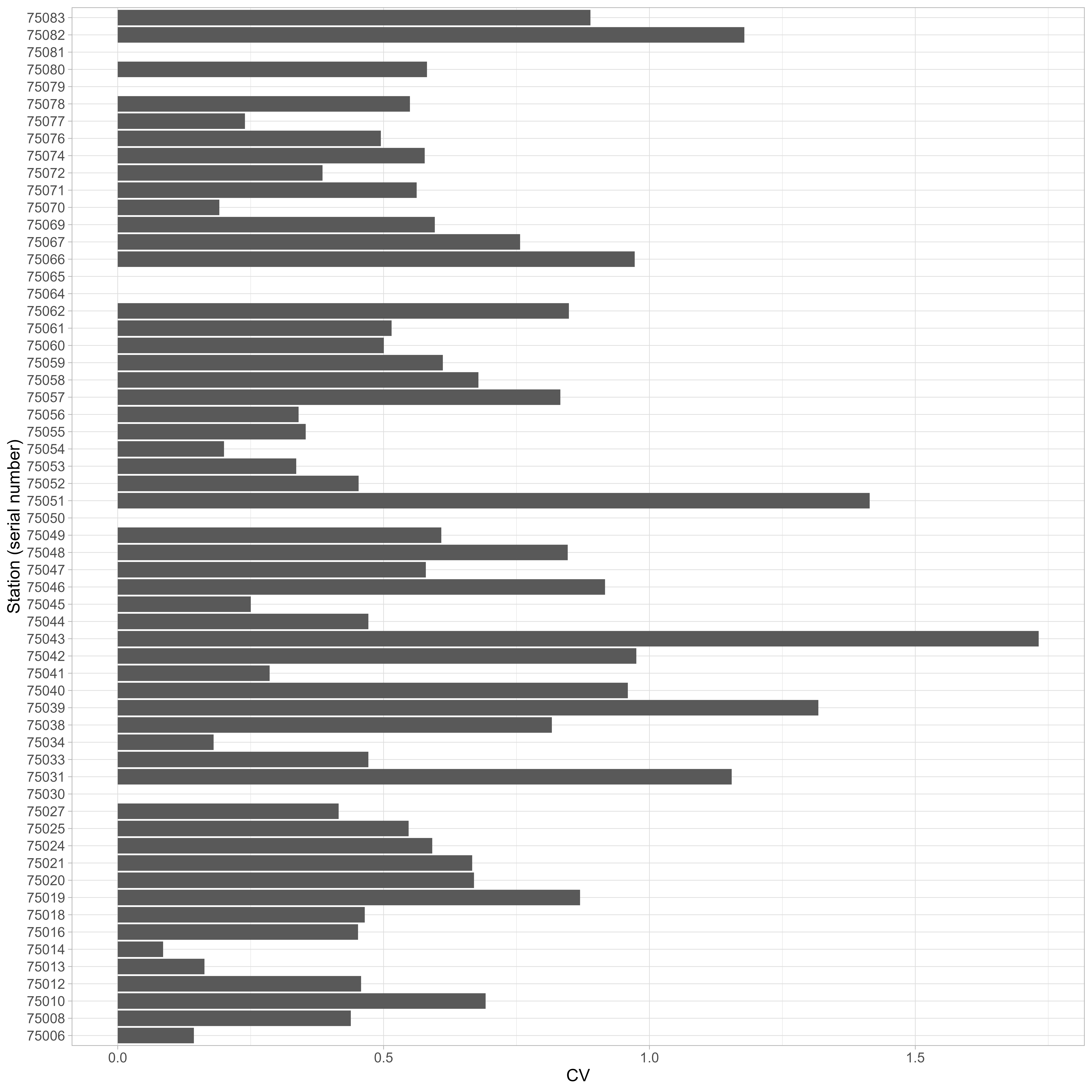
Although scallop annotations resulted in consistent trends in terms of density among persons conducting the annotations and stations (Stokkeland 2023), there were differences in total scallop counts at stations with high scallop densities (Figure 10). Subsequently, coefficient of variation (CV, standard deviation divided by the corresponding mean) among annotations of different counters were relatively high for many stations (Figure 11, with CV > 0.5 for half of the stations and CV > 1 for five stations. Extreme CVs occurred mostly at stations with low densities. The results also highlight substantial intra-transect variation based on patchy distribution. Specific images can therefore contribute much more to the total count than others (Figure 10).
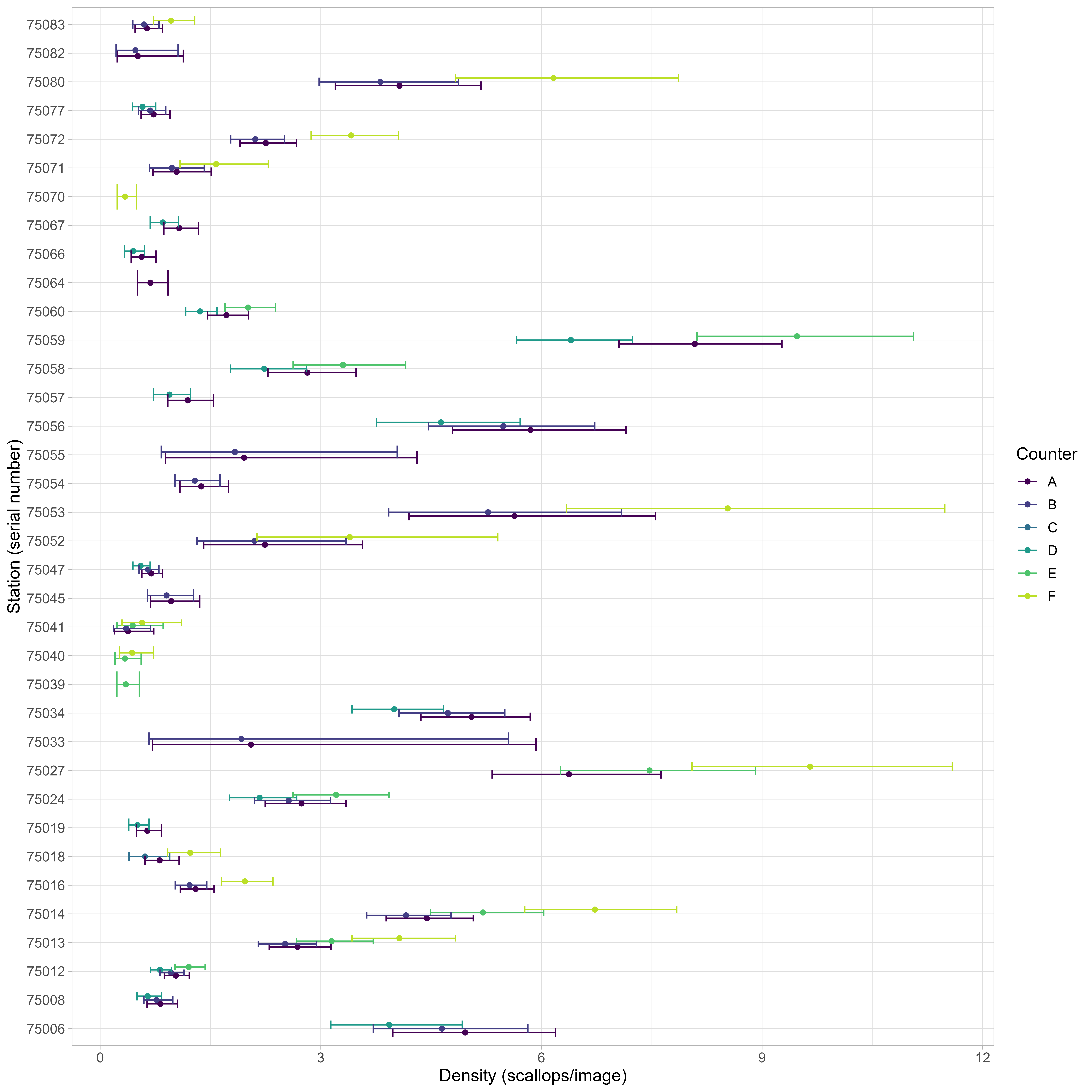
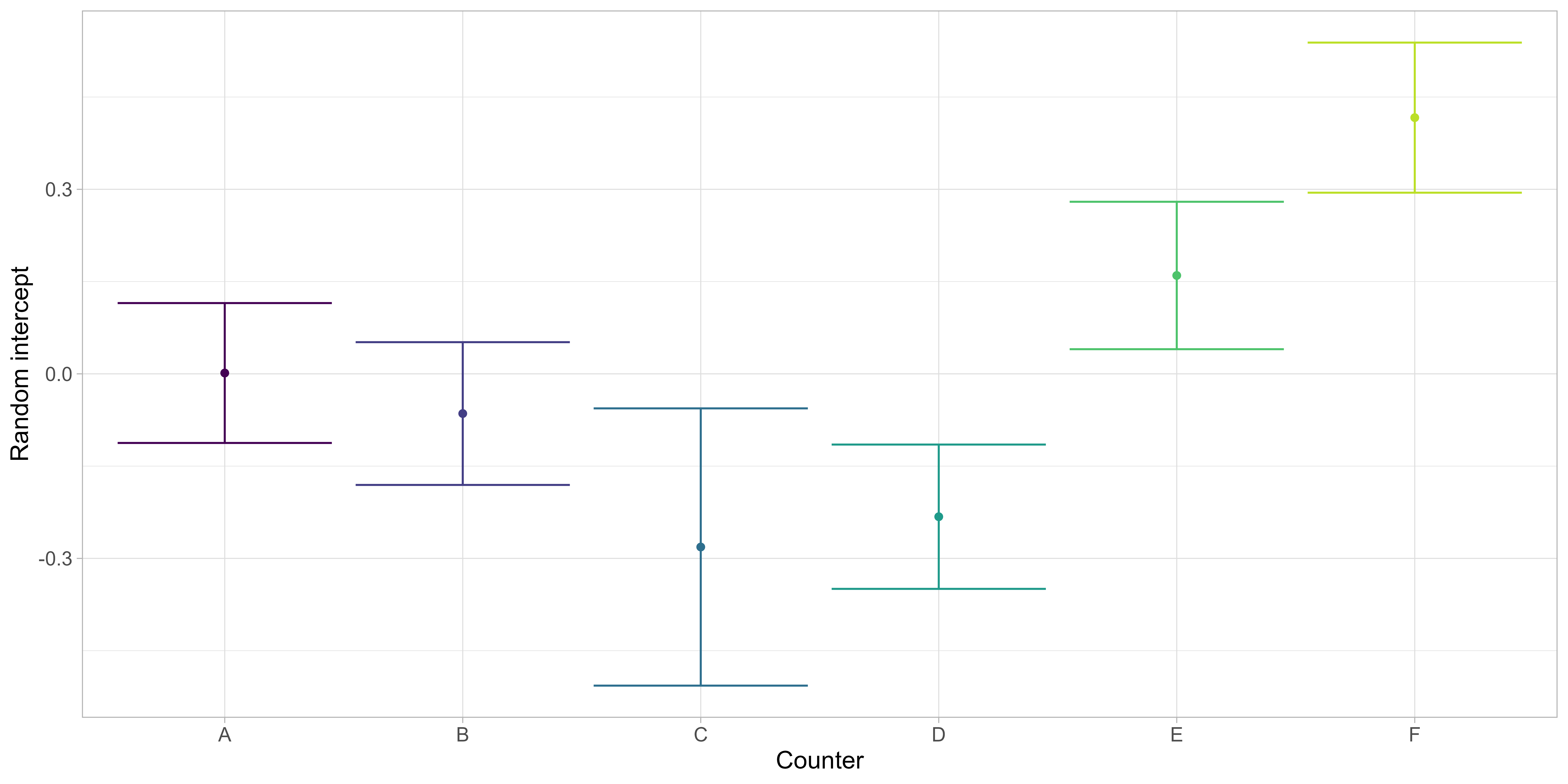
Despite the observed variation, differences in estimated densities per station among counters were not found to be statistically significant (Figure 12). There were relevant random counter effects (Figure 13) with significant differences between the lowest and highest counter effects, indicating some consistently lower or higher numbers of annotated scallops for specific counters. The persons with most experience (“A”) and most stations annotated (“B”) were at or closest to the average, respectively.
Length and age composition
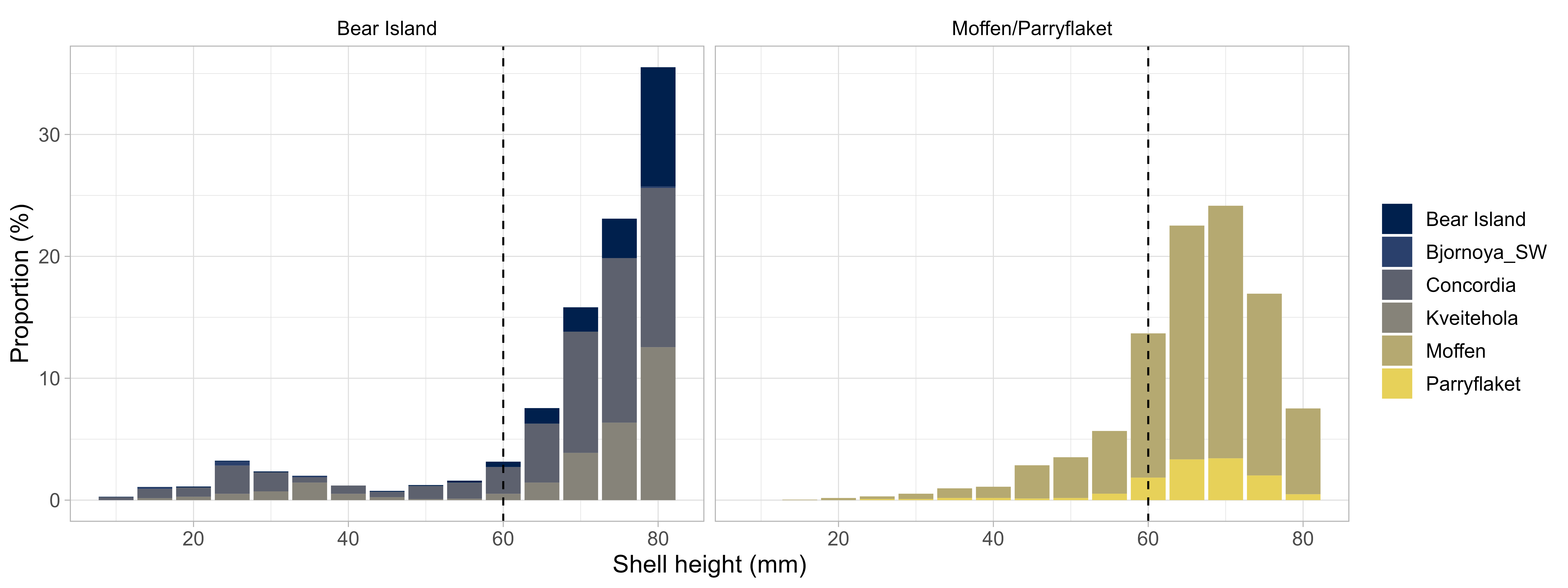
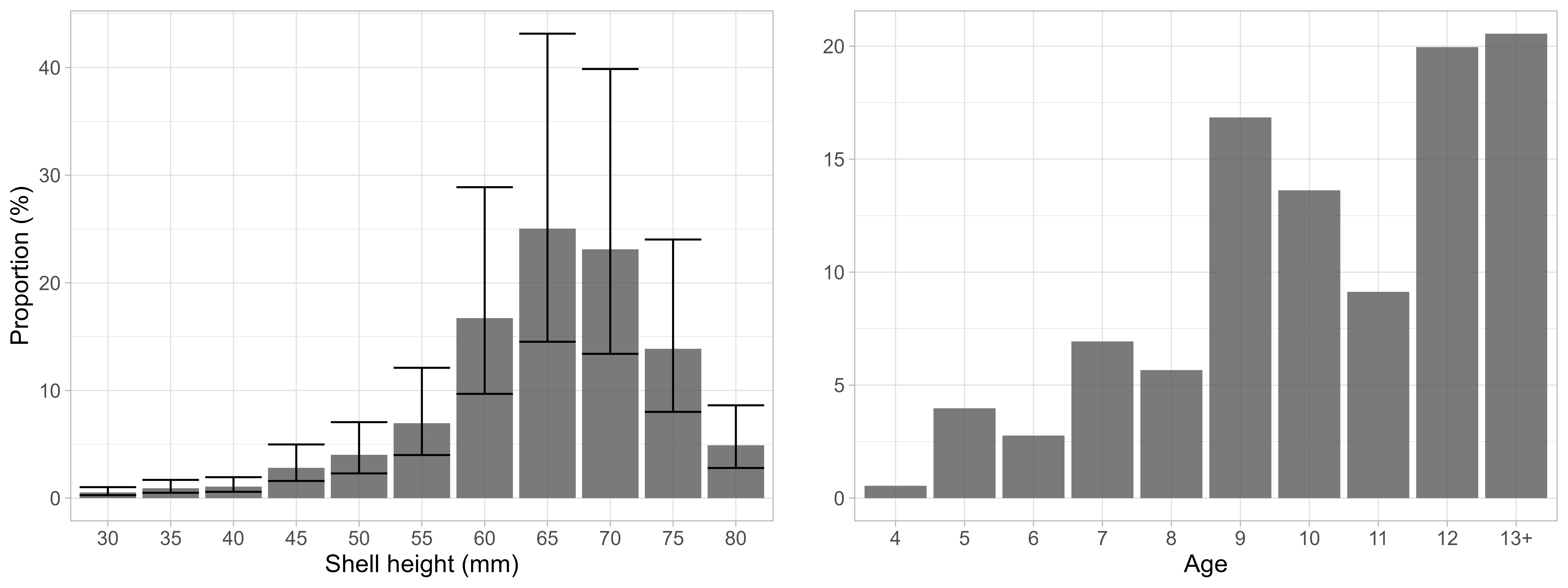
In total, 2273 scallops were measured during the survey in 2022. Of those, 0% were above the MLS of 60 mm shell height. The length frequency distribution was unimodal with a peak at 65-75 mm shell height (Figure 14, right). The scallops on Moffen and Parryflaket were slightly smaller than the ones previously observed on the Bear Island area (Figure 14, left).
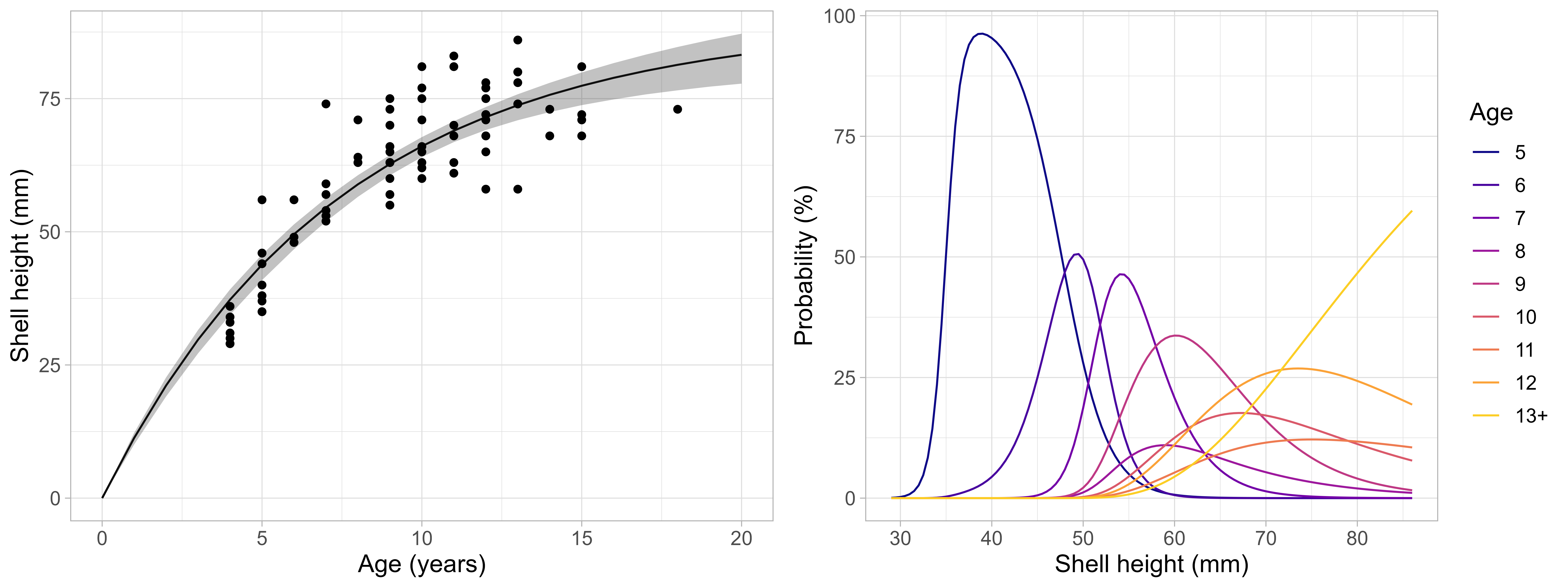
The smaller sizes north of Svalbard were reflected in lower size at age (Figure 15) compared to Bear Island area (Stokkeland 2023). Estimated Von Bertlanffy growth parameters showed more pronounced differences for asymptotic length than growth coefficient, with asymptotic length 89.4 mm and K of 0.14 on Moffen and Parryflaket compared to 91.3 - 105.0mm and 0.12 - 0.21 on Bear Island scallop beds (Sundet & Zimmermann 2020). The probability of being at a specific age was pronounced for small scallops but becomes increasingly flat with higher sizes. Due to the limited sample size of scallops >13 years old, growth curves and age-length keys need to be considered very uncertain for older age classes.
Stock estimates
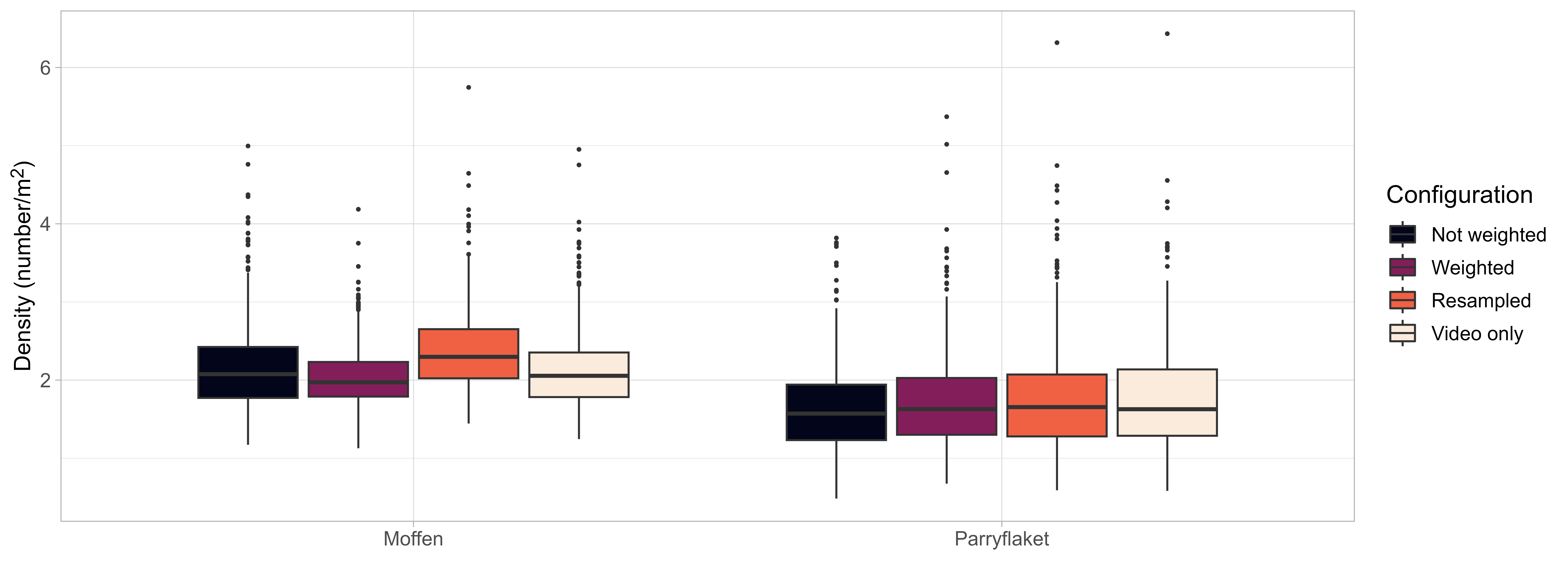
Abundance was estimated based on the selected spatial GAMM implemented with four different configurations aimed at exploring the effects of 1) integrating video and dredge data (in contrast to video data only, see Stokkeland (2023)), 2) weighting scallop densities based on the number of images the are based on, and 3) including counting uncertainty. Estimated mean densities were corresponded well among configurations (Figure 16), with a tendency towards higher density estimates when resampling scallop densities to account for counting uncertainty. This can be attributed to the negative binomial distribution of the scallop count estimates that result in longer upper tail and, thus, a higher probability for scallop counts larger than the mean. Including dredge data had only minor effects compared to video only, while weighting based on number of images increased or decreased precision slightly for large (Moffen) or small (Parryflaket) number of observations, respectively.
Densities on both scallop beds were found to be very similar. Estimated densities ranged between 1.62 and 2.26 scallops/m2 on Moffen and 1.65 and 1.97 on Parryflaket. The results indicate substantial uncertainty in the density estimates, with the 5% percentile of estimated densities as low as 1.00 and the 95% percentile as high as 3.93 scallops/m2 .
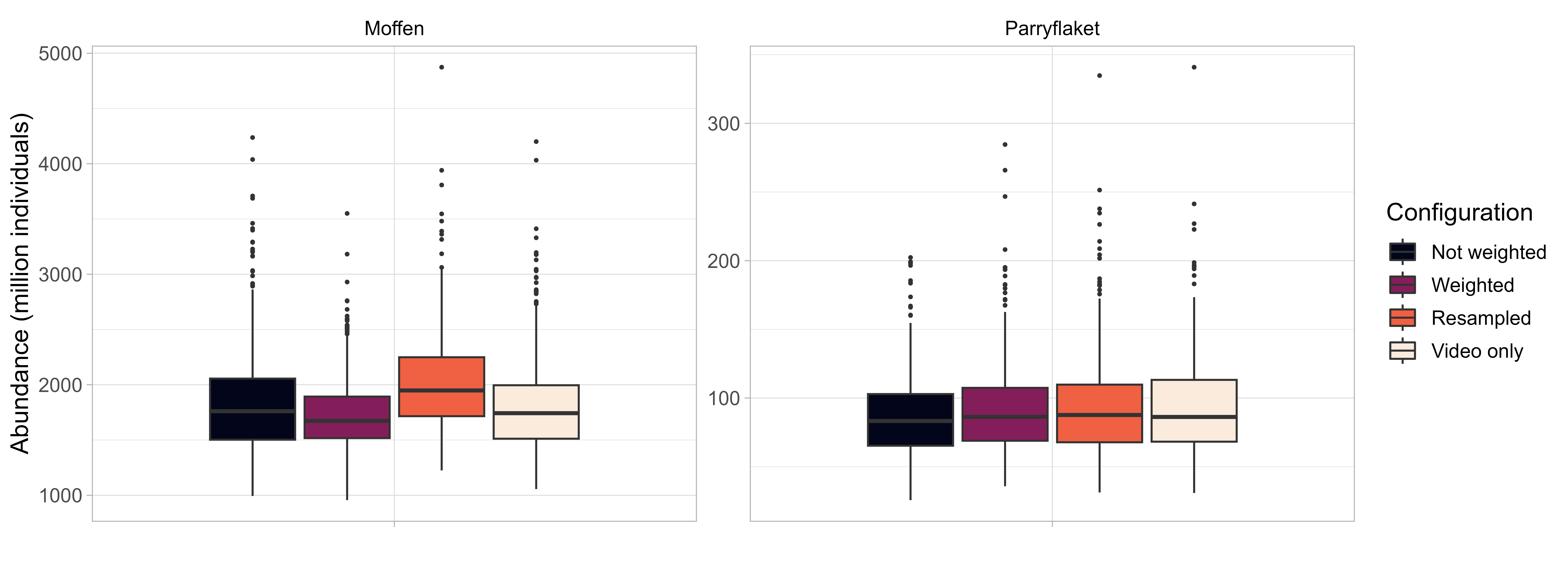
Abundance was calculated as the summed density across space and reflect therefore the density estimates (Figure 17). Because the area on Parryflaket is only 6% of Moffen (53 compared to 848 km2 outside of protected areas), the median total abundance differs between the two scallop beds in the same magnitude: 1510 million on Moffen compared to 87 million on Parryflaket, based on the weighted model using video and dredge data. The total abundance on the two scallop beds north of Svalbard is therefore very similar to the one previously estimated for the three scallop beds in the Bear Island area (Sundet & Zimmermann 2022). The absolute abundance remains, however, very uncertain (Figure 17), especially when accounting for the counting uncertainty.
Length and age frequency based on length-based GAMM integrated with statistical age-length key estimation confirmed that the large majority of scallops was above the minimum landing size of 60mm shell height (Figure 18). Specifically, the estimated mean proportion was 83.7%, in line with the observed length distribution (Figure 14). Accordingly, given an estimated total abundance of 1510 and 87 million on Moffen and Parryflaket, respectively, 1265 and 73 million could be assumed as above minimum landing size.
Genetics
Tissue samples for 98 individual scallops from 13 stations were collected and conserved for population genetic. Processing and analysis are planned.
Contaminants and nutrients
Tissue samples (muscle, hepatopancreas and gonad) from individual scallops were collected at stations 75007, 75009, 75023, 75026, 75028, 75035, 75068, 75073 and analyzed for metals. Composite samples of muscle (n=4), hepatopancreas (HP, n=4) and gonad (n=2, one for each sex) were, in addition, analyzed for persistent organic pollutants including the sums of dioxins and furans (PCDD/F), PCDD/F and dioxin-like PCBs (PCDD/F+dlPCB), and the EU selected non-dioxin like-PCBs (PCB6). Table 1 lists the number of samples collected per station and their location.
In muscle and gonads samples, the levels of lead, mercury and organic pollutants were all below the respective maximum level given for the scallop Pecten maximus (Figure 19). In contrast, high cadmium levels were registered in most individual samples of all tissues, with a mean above the maximum level that applies to the adductor muscle and gonad only (Table 2). The likely source of the unexpectedly high cadmium levels was cross-contamination during on-board sampling or sample preparation. The hepatopancreas in scallops naturally accumulates cadmium to high concentration (Julshamn et al 2008) and cadmium has been shown to be highly mobile with leakage from hepatopancreas to muscle tissue during different treatments in brown crab (Wiech et al 2017). Therefore, further analysis is required to establish the true cadmium concentrations in the different tissues and confirm that cross-contamination caused the high values. As the other analyzed contaminants are less mobile and concentration in HP were higher, it can be assumed that the real values in muscle and gonad are equal or lower to the presented values, even in case of cross-contamination.
| Stratum | Station | Longitude | Latitude | Samples | Composite |
|---|---|---|---|---|---|
| Moffen | 75007 | 15.25 | 80.33 | 10 | 1 |
| Moffen | 75009 | 15.08 | 80.33 | 10 | 1 |
| Moffen | 75023 | 13.97 | 80.26 | 10 | 2 |
| Moffen | 75026 | 13.71 | 80.28 | 10 | 2 |
| Moffen | 75028 | 13.65 | 80.20 | 10 | 3 |
| Moffen | 75035 | 13.48 | 80.21 | 10 | 3 |
| Parryflaket | 75068 | 16.82 | 80.36 | 10 | 4 |
| Parryflaket | 75073 | 16.67 | 80.39 | 10 | 4 |
| Contaminant | Gonade | Hepatopankreas | Muskel |
|---|---|---|---|
| Cadmium (Cd) | 4.658 (±4.7) mg/kg ww | 17.707 (±5.446) mg/kg ww | 3.302 (±2.617) mg/kg ww |
| Mercury (Hg) | 0.018 (±0.015) mg/kg ww | 0.066 (±0.018) mg/kg ww | 0.03 (±0.013) mg/kg ww |
| Lead (Pb) | 0.121 (±0.123) mg/kg ww | 0.267 (±0.104) mg/kg ww | 0.043 (±0.031) mg/kg ww |
| Dioxin (PCDD+PCDF) | 0.059 (±0.016) TEQ2005 pg/g ww | 0.119 (±0.019) TEQ2005 pg/g ww | 0.009 (±0.002) TEQ2005 pg/g ww |
| Dioxin and dl-PCB | 0.069 (±0.017) TEQ2005 pg/g ww | 0.161 (±0.031) TEQ2005 pg/g ww | 0.012 (±0.002) TEQ2005 pg/g ww |
| non-dl-PCB (PCB-6) | 0.474 (±0.001) ng/g ww | 0.918 (±0.055) ng/g ww | 0.082 (±0.023) ng/g ww |
Snow crab expansion
Four stations were surveyed with snow crab pots in Raudfjorden, Woodfjorden and Wijdefjorden, with a soak time of 5 days. No snow crabs were registered. Minor bycatch species such as snails were released.
Conclusion and recommendations
The survey achieved all its aims and covered the targeted scallop beds north of Svalbard comprehensively with a total of 83 stations, including 13 parallel stations with video and dredge. The substantially higher resolution provided a detailed picture of the spatial variation and allowed to explore potential links with environment. The data also underlines the importance of including less suitable habitat to determine distribution limits.
The survey achieved all its aims and covered the targeted scallop beds north of Svalbard comprehensively with a total of 83 stations, including 13 parallel stations with video and dredge. The substantially higher resolution provided a detailed picture of the spatial variation and allowed to explore potential links with environment. The data also underlines the importance of including less suitable habitat to determine distribution limits.
Stock estimates showed high densities and large abundances on Moffen and Parryflaket scallop beds compared to the Bear Island area. The results indicated that estimated abundance on Moffen (outside the protected area) alone is of the same magnitude as the surveyed scallop beds in the Bear Island area. The presented method development underlined the utility of a model-based approach that can capture the spatial variation and uncertainty of estimates better than the design-based approach used in Sundet & Zimmermann (2022). Furthermore, approaches to better incorporate all available data and associated uncertainty into stock estimates performed well and showed overall a consistent picture. We can therefore conclude that it is feasible to calibrate dredge to video data given sufficient overlap between observations, improving the resolution of the available data and possibly allowing for comparisons with historic (dredge-based) survey data. Further parallel stations on future surveys will strengthen the gear calibration approach and allow to explore whether there are gear-specific environmental effects (e.g. bottom depth or substrate).
It can be assumed that the presented stock estimates are conservative because 1) only scallops that could be identified with high confidence as living individuals were counted, 2) impairments of visibility on images (e.g. partly restricted light), potentially obscuring scallops, were not corrected, and 3) repeated annotations reduced the risk of quality issues and improved reproducibility.
Based on the results of the survey, we recommend for future work:
-
Integration of video and dredge data in future distribution and abundance models of Iceland scallops, using weighting to account for the reliability of the underlying data. Historic comparisons with survey data using dredges from before 2019 should be explored to provide indications on long-term changes in the stock.
-
Biological sampling was sufficient to estimate length frequencies and growth, but sampling effort should likely be increased on future surveys or in commercial sampling for more robust estimates, especially for the youngest and oldest age class. Particularly young scallops are difficult to catch and attempts should be made to improve sample numbers. Size- and age-based information is important to understand and model population dynamics and, hence, for management advice.
-
The video sledge used on this survey is easy to deploy, robust and can produce images of sufficient quality. However, the number of images that are good enough to identify scallops confidently was low for many stations, mostly because of the difficulty to tow the sledge slow enough under challenging current conditions. Alternative solutions should be therefore evaluated for future surveys. Given that only still images were used despite recording video, drop cameras could be an alternative. Future development of automated underwater vehicles might also offer the opportunity for more consistent coverage.
-
Comparison of repeated scallop annotations showed the importance of cross-checking and standardization as well as experience when identifying and counting scallops on images or videos. Involvement of multiple people and repeated annotations for at least subsets of the observations are therefore recommended for the future to avoid counter bias.
-
A key delivery of this survey is a library of scallop annotations that should be used to explore machine learning methods to identify scallops on images. Annotation and counting of scallops from video or images are a time-consuming process. Automated techniques may therefore support this task in the future and provide significant gains in efficiency.
-
The survey data including information from protected areas provides an ideal baseline for a before-after-control impact study where the the protected area would serve as control areas in a potential reopening of the scallop beds for harvesting. Especially the very similar densities on Moffen inside and outside the protected area could facilitate a comparative analysis of harvesting impacts on the scallop stock and benthic community. This underlines also the relevance of establishing and using control areas within the entire trial fishery area to ensure a scientifically sound assessment of harvesting impacts.
-
Even though the high cadmium levels registered in most scallop samples were likely the result of cross-contamination, more targeted analysis should be conducted on scallops from this area to clarify whether cadmium concentrations in the different tissues from scallops north of Svalbard are above maximmum limits or to confirm that they were caused by cross-contamination. This should be a priority if a reopening of the Moffen and Parryflaket scallop beds for commercial harvesting will be considered, and contaminant analysis of samples from the current trial fishery area should be conducted for comparison.
-
Contrary to single observations in the past, no snow crab presence inside of the fjords of Northwest-Spitsbergen could be confirmed. This may indicate that potential snow crab occurrences in this area are sporadic or of low density. However, sampling on this survey was limited to four locations and does not allow any comprehensive conclusions on the northwestern spread of snow crab. We recommend continued and more comprehensive monitoring activities to track the likely range expansion of snow crab in the Barents Sea.
Trial fishery
A trial fishery has been approved for the Bear Island Southwest, Kveitehola and Concordia scallop beds in the Bear Island area. In light of the results from the present report, we conclude that:
-
The stock estimates from Moffen and Parryflaket suggest a recovery of the stock and substantial abundances north of Svalbard at or above the level found in the Bear Island area, where a trial fishery started in 2022 (currently limited to five years). Spreading out the fishing effort and total allowable catch of the trial fishery over more scallop beds likely reduces the impact on each scallop bed and, thus, improves overall sustainability from a precautionary perspective. Thus, the inclusion of Moffen and Parryflaket into the trial fishery should be evaluated.
-
The results of this report and Stokkeland (2023) indicate that the boundaries used to delineate the survey areas in 2019, 2020 and 2022 do not necessarily correspond with the distribution range, and there are indications that scallops occur in relevant densities outside of the areas defined here and in Sundet & Zimmermann (2020). Surveying beyond the areas surveyed in 2019, 2020 and 2022 will increase contrast in the data and help to provide better information on the distribution and potential links to environment. In absence of scientific surveys, expanding the trial fishery beyond the currently defined area will improve the information on the (extent of) scallop distribution.
-
Given the novel insights gained here, the advice provided in Sundet & Zimmermann (2020) should be amended with results from this report and Stokkeland (2023). The goal should be an updated management strategy evaluation that 1) includes the scallop beds north of Svalbard, updated stock estimates and biological information with associated uncertainty estimates, and 2) incorporates the spatial stock and fisheries dynamics more explicitly.
Acknowledgements
We thank the crew of RV Helmer Hanssen for their support, and the Norwegian Directorate of Fisheries and Govenor of Svalbard for their cooperation in providing the necessary exemptions. This research was enabled by funding from the Fiskeriforskningsavgift (FFA) and the Norwegian Ministry of Trade, Industry and Fisheries.
References
Anderson, S. C., Ward, E. J., English, P. A., and Barnett, L. A. K. 2022. sdmTMB: an R package for fast, flexible, and user-friendly generalized linear mixed effects models with spatial and spatiotemporal random fields. bioRxiv: 2022.2003.2024.485545. doi: 10.1101/2022.03.24.485545.References
Anderson, S. C., Ward, E. J., English, P. A., and Barnett, L. A. K. 2022. sdmTMB: an R package for fast, flexible, and user-friendly generalized linear mixed effects models with spatial and spatiotemporal random fields. bioRxiv: 2022.2003.2024.485545. doi: 10.1101/2022.03.24.485545.
Bakka, H., Rue, H., Fuglstad, G.-A., Riebler, A., Bolin, D., Illian, J., Krainski, E., et al. 2018. Spatial modeling with R-INLA: A review. WIREs Computational Statistics, 10: e1443. doi: 10.1002/wics.1443.
Breivik, O. N., Aanes, F., Søvik, G., Aglen, A., Mehl, S., and Johnsen, E. 2021. Predicting abundance indices in areas without coverage with a latent spatio-temporal Gaussian model. ICES Journal of Marine Science, 78: 2031-2042. doi: 10.1093/icesjms/fsab073.
Brooks, M., Kristensen, K., van Benthem, K., Magnusson, A., Berg, C. W., Nielsen, A., Skaug, H. J., et al. 2017. glmmTMB Balances Speed and Flexibility Among Packages for Zero-inflated Generalized Linear Mixed Modeling. The R Journal, 9: 378-400
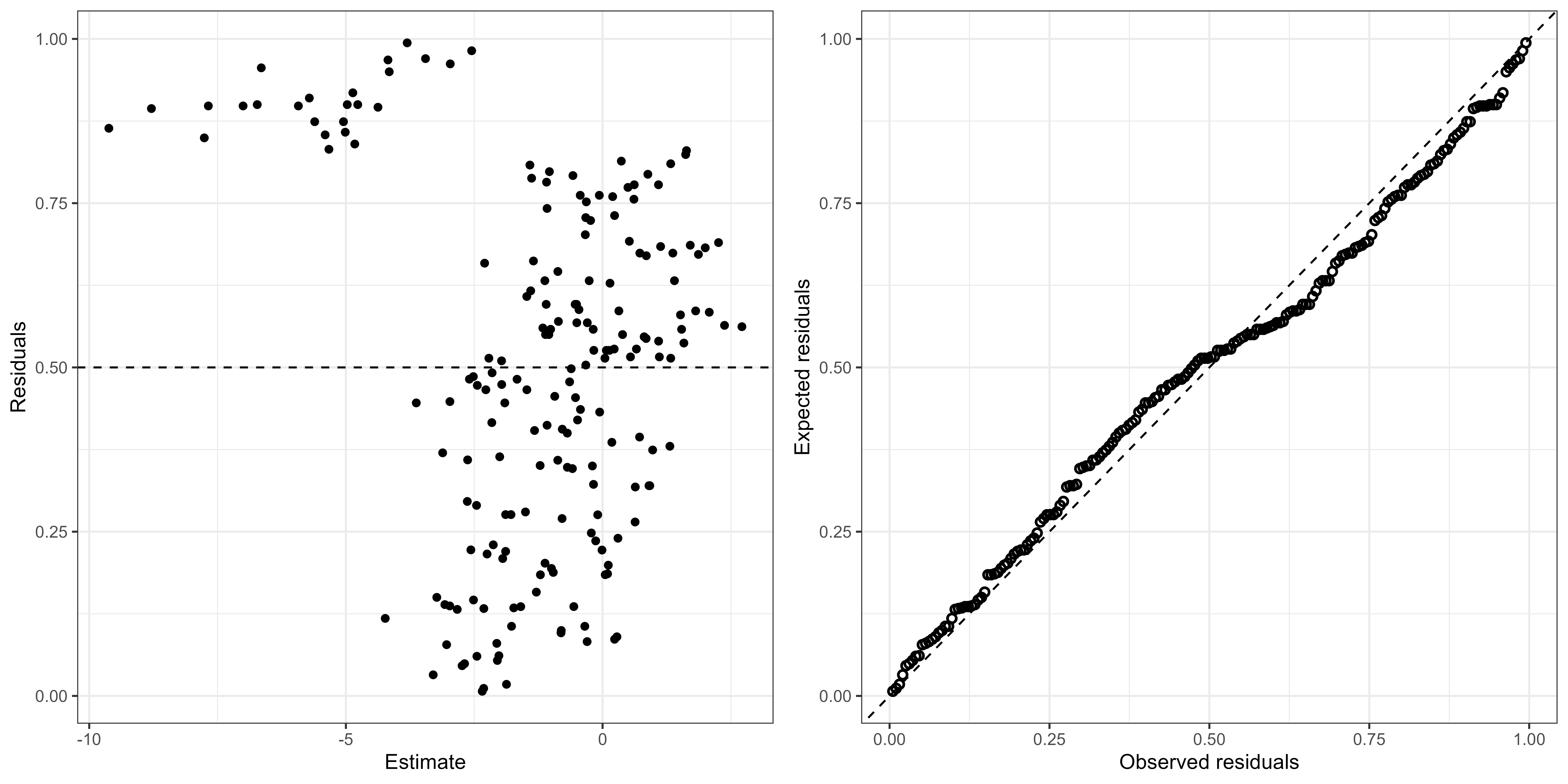
Hartig, F. 2021. DHARMa: Residual Diagnostics for Hierarchical (Multi-Level/Mixed) Regression Models. R package version 0.4.1. edn.
Julshamn, K., Duinker, A., Frantzen, S., Torkildsen, L., & Maage, A. (2008). Organ distribution and food safety aspects of cadmium and lead in great scallops, Pecten maximus L., and horse mussels, Modiolus modiolus L., from Norwegian waters. Bulletin of environmental contamination and toxicology, 80, 385-389. Melsom, A., Counillon, F., LaCasce, J. H. and Bertino, L.: Forecasting search areas using ensemble ocean circulation modeling, Ocean Dyn., 62(8), 1245–1257, doi:10.1007/s10236-012-0561-5, 2012.
Sakov, P., Counillon, F., Bertino, L., Lisæter, K. A., Oke, P. R. and Korablev, A.: TOPAZ4: an ocean-sea ice data assimilation system for the North Atlantic and Arctic, Ocean Sci., 8(4), 633–656, doi:10.5194/os-8-633-2012, 2012.
Stokkeland, M. M. 2023. Improved stock estimation for Iceland scallops (Chlamys islandica) in the Svalbard area. University of Bergen, Bergen, Norway.
Sundet, J. H., and Zimmermann, F. 2020. Stock assessment of Iceland scallops (Chlamys islandica) in the Bear Island area. Rapport fra havforskningen, 27
Vihtakari, M. 2022. ggOceanMaps: Plot Data on Oceanographic Maps using ‘ggplot2’ . R package version 1.3.7. https://mikkovihtakari.github.io/ggOceanMaps
Wickham, H., Averick, M., Bryan, J., Chang, W., McGowan, L. D. A., François, R., Grolemund, G., et al. 2019. Welcome to the Tidyverse. Journal of Open Source Software, 4: 1686
Wiech, M., Vik, E., Duinker, A., Frantzen, S., Bakke, S., & Maage, A. (2017). Effects of cooking and freezing practices on the distribution of cadmium in different tissues of the brown crab (Cancer pagurus). Food Control, 75, 14-20. Zhu, Y., Azad, A. M., Kjellevold, M., Bald, C., Iñarra, B., Alvarez, P., Boyra, G., et al. 2023. Differences in nutrient and undesirable substance concentrations in Maurolicus muelleri across the Bay of Biscay, Norwegian fjords, and the North Sea. Frontiers in Marine Science. doi: https://doi.org/10.3389/fmars.2023.1213612.
Zimmermann, F., Tengvall, J., Strand, H. K., Nedreaas, K., Thangstad, T. H., Husson, B., and Søvik, G. 2023. Fine-scale spatial variation of northern shrimp and Atlantic cod across three Norwegian fjord systems and implications for management. Estuarine, Coastal and Shelf Science. doi: 10.1016/j.ecss.2023.108435.
Annex
Station list
| Station | Serial number | Gear type | Longitude | Latitude | Bottom depth (m) |
|---|---|---|---|---|---|
| 1 | 75001 | Pots | 12.02 | 79.81 | 132 |
| 2 | 75002 | Pots | 13.97 | 79.71 | 132 |
| 3 | 75003 | Pots | 15.30 | 79.73 | 151 |
| 4 | 75004 | Pots | 15.40 | 79.97 | 157 |
| 5 | 75005 | Video | 15.27 | 80.32 | 73 |
| 6 | 75006 | Video | 15.24 | 80.32 | 60 |
| 6 | 75007 | Dredge | 15.25 | 80.33 | 69 |
| 7 | 75008 | Video | 15.11 | 80.32 | 35 |
| 7 | 75009 | Dredge | 15.08 | 80.33 | 33 |
| 8 | 75010 | Video | 14.94 | 80.27 | 33 |
| 8 | 75011 | Dredge | 14.93 | 80.27 | 33 |
| 9 | 75012 | Video | 14.97 | 80.29 | 33 |
| 10 | 75013 | Video | 14.77 | 80.25 | 38 |
| 11 | 75014 | Video | 14.58 | 80.35 | 56 |
| 11 | 75015 | Dredge | 14.61 | 80.34 | 52 |
| 12 | 75016 | Video | 14.48 | 80.31 | 64 |
| 13 | 75017 | Video | 14.40 | 80.28 | 59 |
| 14 | 75018 | Video | 14.33 | 80.20 | 43 |
| 15 | 75019 | Video | 14.12 | 80.25 | 64 |
| 16 | 75020 | Video | 14.12 | 80.32 | 70 |
| 17 | 75021 | Video | 14.22 | 80.36 | 97 |
| 18 | 75022 | Video | 13.91 | 80.26 | 70 |
| 18 | 75023 | Dredge | 13.97 | 80.26 | 72 |
| 19 | 75024 | Video | 13.88 | 80.23 | 62 |
| 20 | 75025 | Video | 13.67 | 80.28 | 84 |
| 20 | 75026 | Dredge | 13.71 | 80.28 | 82 |
| 21 | 75027 | Video | 13.64 | 80.20 | 55 |
| 21 | 75028 | Dredge | 13.65 | 80.20 | 55 |
| 22 | 75029 | Video | 13.34 | 80.24 | 69 |
| 23 | 75030 | Video | 13.16 | 80.24 | 111 |
| 24 | 75031 | Video | 13.21 | 80.17 | 99 |
| 24 | 75032 | Dredge | 13.23 | 80.17 | 100 |
| 25 | 75033 | Video | 13.28 | 80.21 | 74 |
| 26 | 75034 | Video | 13.45 | 80.22 | 48 |
| 26 | 75035 | Dredge | 13.48 | 80.21 | 47 |
| 27 | 75036 | Video | 13.41 | 80.15 | 76 |
| 28 | 75037 | Video | 13.58 | 80.13 | 65 |
| 29 | 75038 | Video | 13.89 | 80.07 | 54 |
| 30 | 75039 | Video | 14.11 | 80.02 | 38 |
| 31 | 75040 | Video | 14.31 | 79.97 | 60 |
| 32 | 75041 | Video | 14.72 | 79.95 | 100 |
| 33 | 75042 | Video | 14.78 | 79.91 | 85 |
| 34 | 75043 | Video | 14.84 | 80.03 | 50 |
| 35 | 75044 | Video | 15.16 | 80.19 | 36 |
| 36 | 75045 | Video | 16.78 | 80.34 | 90 |
| 37 | 75046 | Video | 15.21 | 80.27 | 25 |
| 38 | 75047 | Video | 15.24 | 80.32 | 66 |
| 39 | 75048 | Video | 14.64 | 80.39 | 60 |
| 40 | 75049 | Video | 14.41 | 80.40 | 59 |
| 41 | 75050 | Video | 14.65 | 80.00 | 33 |
| 42 | 75051 | Video | 14.26 | 80.00 | 27 |
| 43 | 75052 | Video | 13.92 | 80.03 | 81 |
| 44 | 75053 | Video | 13.84 | 80.13 | 40 |
| 45 | 75054 | Video | 14.32 | 80.19 | 41 |
| 46 | 75055 | Video | 13.91 | 80.16 | 44 |
| 47 | 75056 | Video | 13.68 | 80.17 | 50 |
| 48 | 75057 | Video | 13.45 | 80.15 | 71 |
| 49 | 75058 | Video | 13.37 | 80.20 | 73 |
| 50 | 75059 | Video | 13.54 | 80.19 | 52 |
| 51 | 75060 | Video | 13.25 | 80.26 | 70 |
| 52 | 75061 | Video | 13.22 | 80.31 | 82 |
| 53 | 75062 | Video | 13.47 | 80.28 | 89 |
| 36 | 75063 | Dredge | 16.80 | 80.34 | 93 |
| 54 | 75064 | Video | 16.83 | 80.33 | 79 |
| 55 | 75065 | Video | 16.95 | 80.31 | 104 |
| 56 | 75066 | Video | 17.00 | 80.33 | 54 |
| 57 | 75067 | Video | 16.78 | 80.36 | 62 |
| 57 | 75068 | Dredge | 16.82 | 80.36 | 68 |
| 58 | 75069 | Video | 16.89 | 80.37 | 42 |
| 59 | 75070 | Video | 17.10 | 80.43 | 40 |
| 60 | 75071 | Video | 16.76 | 80.43 | 42 |
| 61 | 75072 | Video | 16.67 | 80.39 | 58 |
| 61 | 75073 | Dredge | 16.67 | 80.39 | 50 |
| 62 | 75074 | Video | 15.12 | 80.26 | 26 |
| 62 | 75075 | Dredge | 15.14 | 80.26 | 27 |
| 63 | 75076 | Video | 14.90 | 80.23 | 31 |
| 64 | 75077 | Video | 14.54 | 80.31 | 64 |
| 65 | 75078 | Video | 14.15 | 80.32 | 78 |
| 66 | 75079 | Video | 13.89 | 80.30 | 94 |
| 67 | 75080 | Video | 13.74 | 80.23 | 60 |
| 68 | 75081 | Video | 13.56 | 80.26 | 72 |
| 69 | 75082 | Video | 13.88 | 80.20 | 49 |
| 70 | 75083 | Video | 13.72 | 80.14 | 39 |
Mesh
Model selection and validation
| Formula | AICc | deltaAICc | AICscore | AICweight |
|---|---|---|---|---|
| fStratum + fGeartype + s(depth, k = 3) | 444 | 0.00 | 1.00 | 0.56 |
| fStratum + fGeartype + s(depth, k = 3) + s(mlp, k = 3) | 446 | 1.89 | 0.39 | 0.22 |
| fStratum + fGeartype + s(depth, k = 3) + s(velocity, k = 3) | 449 | 4.31 | 0.12 | 0.07 |
| fStratum + fGeartype + s(depth, k = 3) + s(btemp, k = 3) | 449 | 4.37 | 0.11 | 0.06 |
| fStratum + fGeartype + s(depth, k = 3) + s(btemp, k = 3) + s(mlp, k = 3) | 450 | 5.29 | 0.07 | 0.04 |
| fStratum + fGeartype + s(depth, k = 3) + s(mlp, k = 3) + s(velocity, k = 3) | 450 | 5.56 | 0.06 | 0.03 |
| fStratum + fGeartype + s(depth, k = 3) + s(btemp, k = 3) + s(velocity, k = 3) | 453 | 8.73 | 0.01 | 0.01 |
| fStratum + fGeartype + s(depth, k = 3) + s(btemp, k = 3) + (mlp, k = 3) + s(velocity, k = 3) | 454 | 9.14 | 0.01 | 0.01 |
Bear Island area: distribution and stock estimates