Torsk og hyse i Barentshavet er verdens største bestander av disse fiskearten, og forvaltes og overvåkes av Norge i samarbeid med Russland. For å kunne beregne kvoter og forvalte artene bærekraftig trenger vi data fra tokt. Økosystemtoktet i Barentshavet er havforskningsinstituttets mest omfattende tokt og gjennomføres årlig i samarbeid Polar Branch of FSBIU VINRO. I denne rapporten beregner vi indekser for torsk og hyse med programvaren StoX som er utviklet ved Havforskningsinstituttet.
StoX applied to cod and haddock data from the Barents Sea NOR-RUS ecosystem cruise in autumn
— Swept area abundance, length and weight at age 2004-2017
Report series:
Fisken og havet 2019-6
ISSN: 1894-5031
Published: 11.12.2019
Updated: 12.12.2019
Project No.: 83630, 2019113, 14809, 83093
Research group(s):
Demersal fish,
Ecosystem acoustics,
The Norwegian Marine Data Centre (NMD)
Program:
The Barents Sea and Arctic Ocean Ecosystems
Approved by:
Research Director(s):
Geir Huse
Program leader(s):
Maria Fossheim
Norsk sammendrag
Summary
North East Arctic cod and haddock are the largest stocks of these species in the world. Data from the Barents Sea NOR-RUS ecosystem cruise (BESS) in autumn is used as input to the assessment of these species. Here, we used the StoX software to recalculate the indices from the survey. First, we stratified the area covered by BESS into nine strata based on average cod and haddock density and modified this strata system by year to account for year to year variation in spatial coverage and survey design). We then used these strata systems to estimate swept area abundance indices, weights and lengths at age. We evaluated the quality of the indices based on uncertainty estimates and internal consistency. Coefficient of Variation (CV) from bootstrap runs was used as a measure of uncertainty. Low CV indicates that the number of samples are adequate relative to the abundance and patchiness of the targeted species. Consistency is the relationship between the abundance of a cohort at age a in year y with the abundance of the same cohort later at older ages. The indices for a cohort should decline over time due to natural and fishing mortality (assuming adequate size/age dependent fishing efficiency correction and adequate spatial coverage of all ages). The correlation between the log abundance of a cohort at age a in year y with log abundance of the same cohort at age a+1 (of ages used in tuning) in year y+1 were ≥0.73 for cod and ≥0.74 for haddock. The CVs were much higher for haddock than for cod, still internal consistencies were about similar for the two species. The CVs increased with age, especially for cod. There appear to be problems with haddock sampling, demonstrated by the very high CVs especially in 2016, a year with lack of coverage in the south-east, where most of the haddock was distributed. We recommend keeping the survey design of BESS the same every year. If changes are made to the design, sampling or gear, these changes should first be carefully considered and then documented. Survey indices for haddock could probably be improved by using a denser station grid in the main haddock distribution area, this will require more survey days. “Holes” and inadequate spatial extent of the survey strongly reduces the quality of the data, are difficult to adjust for and should be avoided.
1 - Introduction
North East Arctic (NEA) cod ( Gadus morhua ) and NEA haddock ( Melanogrammus aeglefinus ) are the largest stocks of these species in the world and have great economic value. In 2018, the Norwegian catches alone had a first-hand landing value of over 8 billion NOK. Indices from three surveys are used for the catch advice of both these stocks: the “ Barents Sea NOR-RUS ecosystem cruise in autumn” (BESS) , the “ Barents Sea NOR-RUS demersal fish cruise in winter” (winter survey), and the Russian bottom trawl survey for demersal fish (Lepesevich and Shevelev 1997, discontinued after 2017). Indices from these surveys are used as tuning series for cod ages 3-12 and haddock ages 3-9 in the stock assessment models (SAM, www.stockassessment.org ) and the indices for pre-recruits are used as input to the recruitment forecast models (ICES 2019).
StoX is a software developed at the Institute of Marine Research for marine survey analysis and index calculation. StoX is available for free ( ftp://ftp.imr.no/StoX/Download/ ) and is relatively well documented (Johnsen et al 2019). StoX is currently used for bottom trawl index calculation from winter survey data (Mehl et al 2016) but not from BESS data. BESS indices for cod and haddock are calculated with the BIOFOX software developed and run by the Polar Branch of FSBIU VINRO, Murmansk Russia (Prozorkevich and Gjøsæter 2014). Here we use StoX to calculate BESS swept area indices for haddock and cod 2004-2017. StoX needs a predefined strata system to estimate swept area indices. Whereas the winter survey has had a predefined strata system and a stratified survey design since the onset in 1981, BESS, starting in 2004, has had no predefined strata system. BESS has employed a regular grid design, with notable deviations, especially in deeper areas and around Svalbard.
Here we develop a strata system and use the StoX software to estimate haddock and cod abundance indices from “Barents Sea NOR-RUS ecosystem cruise in autumn”.
2 - Methods
2.1 - Input data and strata system
BESS started as a compilation and extension of several surveys with different aims, gears and survey designs. BESS has been running annually August – October 2004-2018 with 2-3 Norwegian vessels and 1-2 Russian vessels (Appendix Table 1). The number of survey days and the number of bottom trawl stations has declined over the years (Appendix Table 1). With the exceptions shown and described in Appendix Figures 1-15, the whole Barents Sea shelf has been covered with stations set out in a regular grid with inter-station distance of 35 nautical miles. From 2017 and onwards the stations in the station grid was set out using the Albers equal-area projection. We do not include data from 2018 further due to a nearly complete lack of coverage in the eastern Barents Sea (Appendix Figure 15). The 2018 BESS indices were not used in the assessment (ICES 2019). BESS monitors plankton, oceanographic conditions, pelagic and demersal fish, pollution, benthos, shellfish, sea birds and marine mammals using an array of sampling methods. Here we used only data from bottom trawls. The standard towing time for bottom trawls is 15 minutes at 3 knots, but in deeper areas along the shelf break, tows has been longer due to lower fish densities. The bottom trawl gear, rigging, handling of the catches etc are similar as for the winter survey and are detailed in Mehl et al (2016, see also Appendix Table 2). The exception is that from 2018 and onwards gonadal weights and stages have not been registered at BESS. The number of aged and length measured cod and haddock is shown in Appendix Table 1.
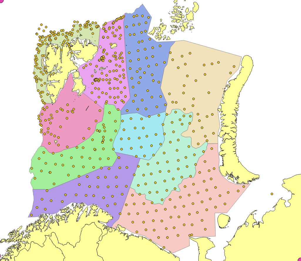
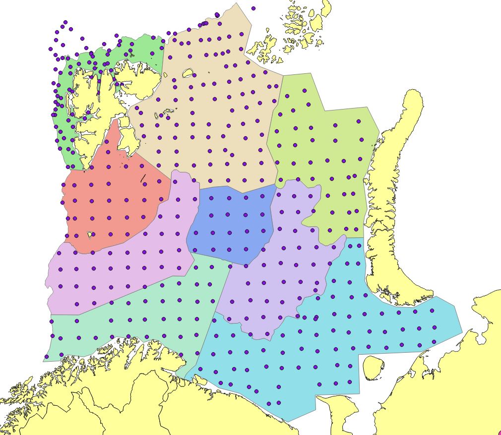
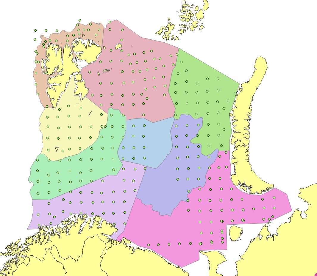
Strata are used in StoX when filling in missing ages for length groups and in bootstrapping (see below). The strata should therefore ideally be homogenous with respect to the relationships between age and length and age and weight, as well as age specific abundances. We defined a basic strata system from the geographical distribution patterns of cod and haddock, observed at BESS and aggregated over the period 2009-2018 (Figure 1).
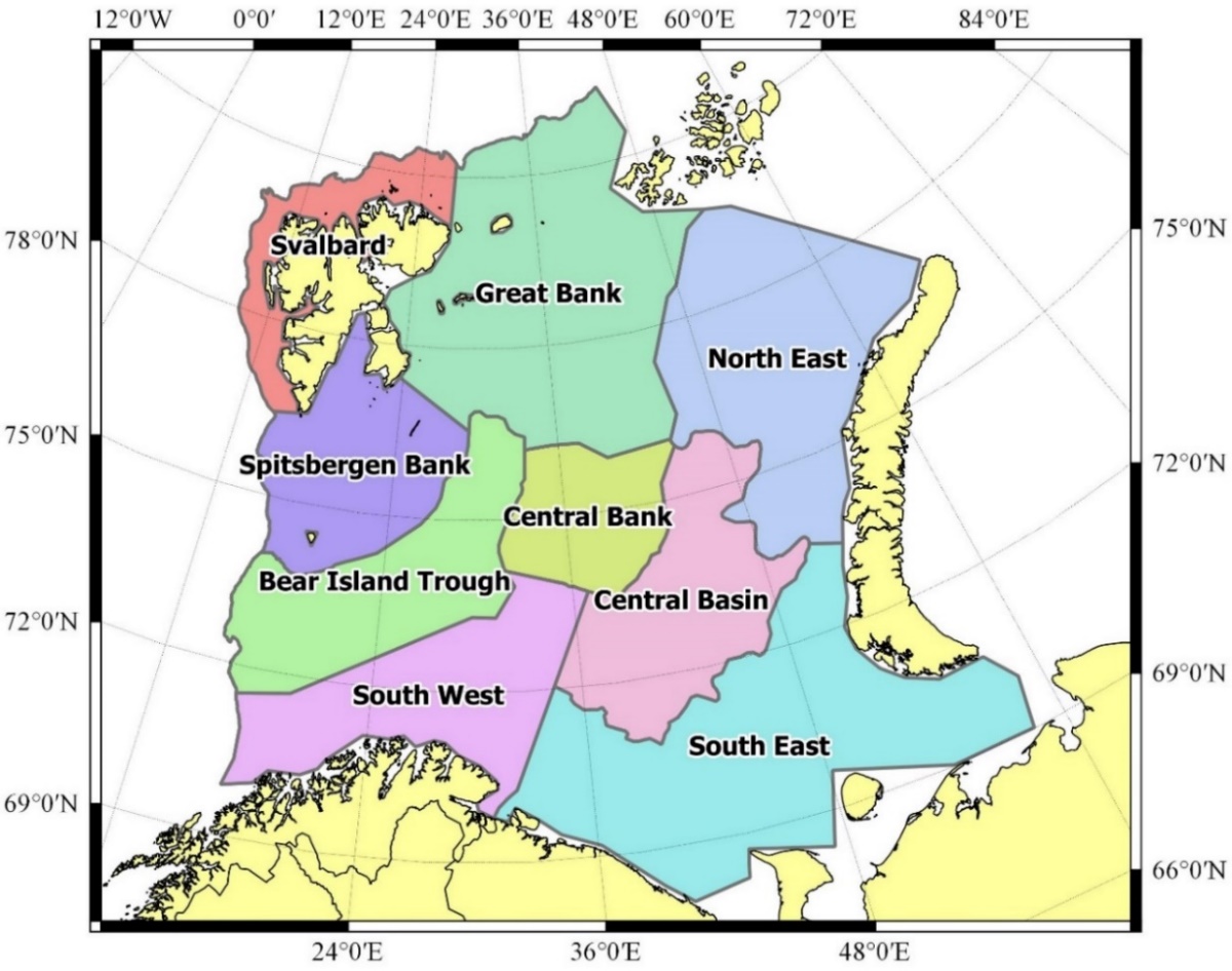
Figure 1. The basic BESS strata system used here with modifications by year accounting for the variable coverage and station densities in some areas and years (Appendix Figures).
The 250 m depth contour was used as guideline for the borders between strata, as a preliminary analysis show that this depth separates quite well between low (deeper) and high-density (shallower) areas for cod and haddock. The 500 m depth contour was used as a limit for the strata system towards the Norwegian Sea in the West and the Polar Ocean to the North as the densities of cod and haddock at greater depths are very low. The southernmost strata were divided by the border separating the Russian-Norwegian Exclusive zones, since the survey effort varied between Russian and Norwegian vessels in this area some years.
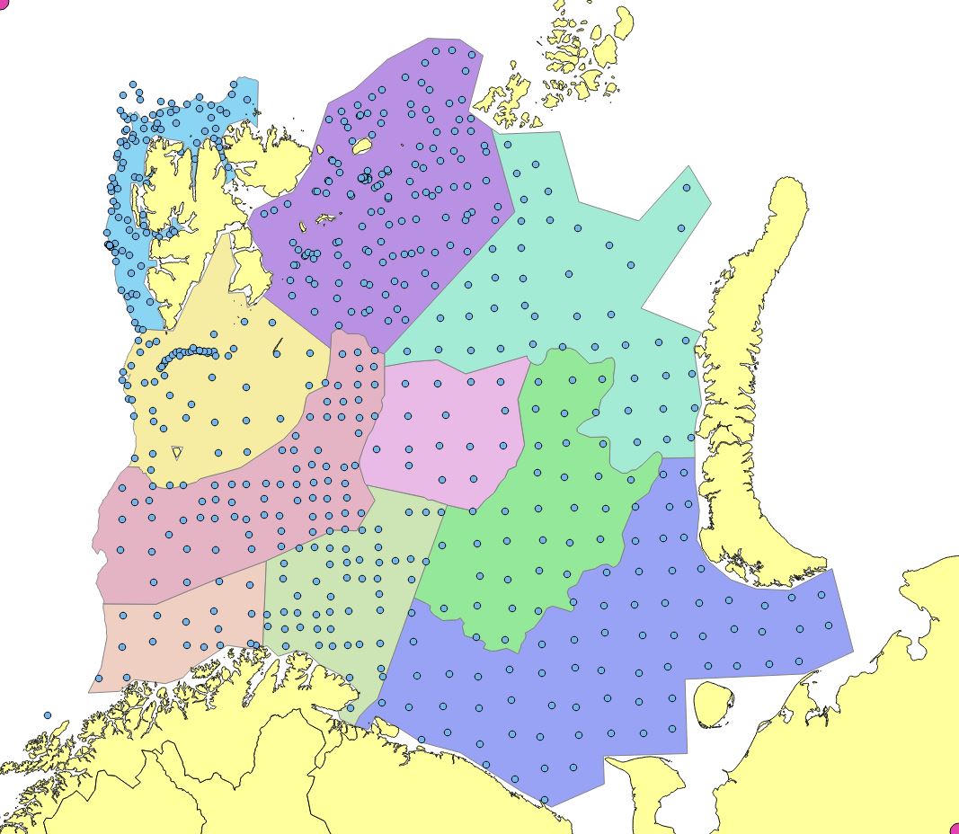
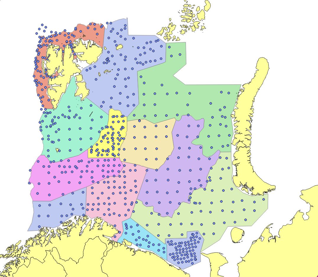
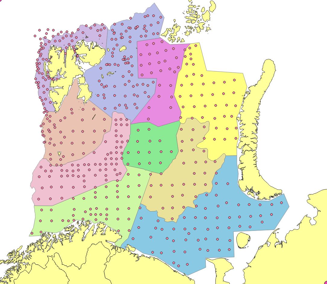
The result is a basic strata system that served as a starting point when generating the yearly strata systems used for estimation (Figure 1), modified to account for irregular sampling, ice hindrance, and limited survey coverage due to other reasons (Appendix Figures 1-15). The size of the strata was defined so that each stratum ideally contained at least 20 trawl hauls (although difficult to satisfy some years). We also modified the basic strata system to account for area specific differences in station density, since if not, areas with denser station coverage grid will be given more weight when calculating totals for the whole area.
2.2 - StoX calculations and settings
The data was downloaded from: https://datasetexplorer.hi.no/apps/datasetexplorer/v2/navigation and the folder “cruise series\Barents Sea NOR-RUS ecosystem cruise in autumn”.
The StoX projects presented here is stored in folders:
Surveytimeseries\Barents Sea Northeast Arctic haddock bottom trawl index in autumn
Surveytimeseries\Barents Sea Northeast Arctic cod bottom trawl index in autumn
We used the same station filter in StoX to select stations as Mehl et al (2016), except that stations with the gear code “3293” (“Tromsø rigging”) was included in the StoX filter here (Tromsø rigging is used for bottom trawls at soft bottoms and is described in Mehl et al 2016 and in Appendix Table 2).
Furthermore, we used 1 cm length groups rather than 5 cm length groups as in Mehl et al (2016) when applying the length dependent sweep width correction. The equations for length dependent sweep width for cod and haddock can be found in Mehl et al (2016).
2.2.1 - Swept area indices by length
The swept area density ( ρ , individuals per square nautical mile, inds nmi -2 ) by stratum (k), station (s) and length group l (1 cm), is given by
 , (eqn 1)
where f k,s,l is the number of individuals standardized over a towing distance of 1 nmi by k, s and l, and sw l is the adjusted swept width in nmi’s by length group calculated using
 , (eqn 2)
where EW l is the length dependent effective swept width
The abundance ( N , inds) by l and k is calculated using
 (eqn 3)
where A is stratum area (nmi 2 ), and ρ k,l is the average swept area density by l and k, given by
 (eqn 4)
where n is number of stations.
2.2.2 - Swept area indices by age
The sampling protocol for the BESS survey is to sample one individual from each 5 cm length group at each trawl station for aging and individual weights. A two-stage conversion process is used to convert the abundance of fish by length group to abundance of fish by age group.
Firstly, the abundance ( N k,l ) by length group l (5 cm) and stratum k is distributed the length-measured individuals (j) to generate so-called “Super-individuals” (super-individuals represent fractions of a total, our use corresponds to a probability based design where  is the inverse of the inclusion probability for a single fish sample), each representing an abundance estimated as:
 , (eqn 5)
where
 (eqn 6)
and m is the number of length-measured individuals
Secondly, in instances where a super-individual is not aged, the missing age is filled in by a random data imputation. The imputation of missing age is principally carried out at the station level, randomly selecting the value from aged super-individuals within the same length group. If no aged super-individual is available at the station level, the imputation is attempted at strata level, or lastly on survey level. In instances where no age information is available at any level for a specific length group, the abundance estimate is presented with unknown age (Johnsen et al 2019).
2.2.3 - Length and weight at age
Length and weight at age was calculated using the weighting factors defined in eqn 6 (the “super -individuals”).
2.2.4 - Uncertainty and consistency of abundance indices
Uncertainty was estimated as the coefficient of variation (ratio of standard deviation to the mean, CV). StoX calculates CV using bootstrap runs by stratum, treating each trawl station as the primary sampling unit. Here we used 500 bootstrap runs
Consistency was quantified here as the correlation between the log abundance of all cohorts at age a in year y with the log abundances of the same cohort at older ages and later years. It is most common to consider only the correlation between the abundance of the cohorts at age a in year y, with the abundance at age a+1 in y+1, but here we present the correlations for the cohorts at all ages.
3 - Results
3.1 - Estimates at age
3.1.1 - Abundance at age
The numbers at ages in millions are given for cod and haddock in Table 1 and 2 respectively.
Table 1. Cod numbers at age in millions, swept area estimates, mean values from 500 bootstraps.
| Year | 1 | 2 | 3 | 4 | 5 | 6 | 7 | 8 | 9 | 10 | 11 | 12 | 13 | 14 | 15 | 16+ |
| 2004 | 410.02 | 290.99 | 91.39 | 281.28 | 155.27 | 75.82 | 40.30 | 10.51 | 1.97 | 0.56 | 0.12 | 0.05 | - | 0.16 | - | - |
| 2005 | 359.91 | 124.19 | 178.94 | 35.00 | 96.52 | 31.15 | 18.43 | 6.89 | 1.79 | 0.80 | 0.13 | - | 0.09 | - | - | - |
| 2006 | 454.91 | 432.85 | 142.67 | 121.00 | 36.91 | 47.49 | 16.88 | 8.34 | 3.32 | 0.46 | 0.30 | 0.03 | - | - | - | - |
| 2007 | 301.31 | 302.69 | 301.65 | 76.16 | 47.49 | 9.23 | 16.47 | 3.29 | 1.30 | 0.31 | - | 0.29 | - | 0.05 | - | - |
| 2008 | 107.26 | 266.04 | 342.90 | 350.48 | 89.60 | 47.01 | 10.08 | 15.35 | 3.39 | 0.87 | 0.38 | 0.18 | 0.08 | - | - | 0.08 |
| 2009 | 538.89 | 71.40 | 213.65 | 236.63 | 357.16 | 128.46 | 27.58 | 10.63 | 8.18 | 2.62 | 0.85 | 0.30 | 0.17 | - | - | - |
| 2010 | 383.76 | 87.13 | 59.89 | 151.12 | 448.60 | 513.28 | 160.50 | 39.71 | 10.52 | 7.21 | 2.05 | 0.28 | 0.26 | 0.21 | - | - |
| 2011 | 378.05 | 150.56 | 112.78 | 95.19 | 218.77 | 319.56 | 214.58 | 29.86 | 7.71 | 1.84 | 1.35 | 0.65 | 0.29 | - | - | - |
| 2012 | 1301.35 | 245.25 | 170.88 | 131.23 | 77.53 | 189.52 | 162.84 | 99.89 | 12.83 | 3.98 | 1.60 | 1.33 | 0.41 | 0.14 | 0.18 | - |
| 2013 | 677.38 | 670.39 | 250.75 | 147.61 | 110.09 | 50.77 | 120.36 | 131.36 | 56.14 | 7.68 | 2.98 | 1.92 | 0.35 | 0.38 | 0.12 | - |
| 2014* | 264.91 | 117.48 | 175.73 | 94.18 | 82.07 | 41.56 | 17.25 | 32.55 | 19.73 | 8.00 | 2.21 | 0.79 | 0.53 | 0.09 | 0.10 | 0.07 |
| 2015 | 600.35 | 178.31 | 184.19 | 219.08 | 148.61 | 61.65 | 61.53 | 32.26 | 35.71 | 25.22 | 7.68 | 1.42 | 0.19 | 0.89 | - | 0.06 |
| 2016 | 394.23 | 386.08 | 82.06 | 101.12 | 128.70 | 73.23 | 42.64 | 26.19 | 12.86 | 11.21 | 4.37 | 1.37 | 0.35 | 0.65 | 0.08 | 0.23 |
| 2017 | 744.28 | 203.72 | 356.39 | 94.29 | 68.18 | 139.29 | 72.95 | 27.24 | 11.80 | 5.18 | 4.67 | 4.00 | 1.72 | 0.81 | 0.33 | - |
*2014 not used in cod assessment due to poor coverage of the Northern Barents Sea, see App. Fig 11.
Table 2 Haddock numbers at age in millions, swept area estimates, mean values from 500 bootstraps.
| Year | 1 | 2 | 3 | 4 | 5 | 6 | 7 | 8 | 9 | 10 | 11 | 12 | 13+ |
| 2004 | 149.12 | 237.63 | 124.05 | 53.53 | 46.42 | 24.68 | 2.03 | 1.75 | - | 0.16 | - | 0.05 | 0.14 |
| 2005 | 575.23 | 92.64 | 292.08 | 133.23 | 14.24 | 30.11 | 10.19 | 0.33 | 0.45 | 0.20 | 0.10 | 0.08 | - |
| 2006 | 2190.94 | 872.46 | 79.60 | 99.57 | 41.93 | 9.69 | 12.11 | 4.46 | 0.58 | 1.49 | 0.06 | 0.07 | - |
| 2007 | 869.81 | 978.81 | 511.18 | 45.27 | 36.41 | 7.04 | 1.36 | 3.02 | 7.23 | 0.43 | 0.11 | 0.11 | 0.09 |
| 2008 | 333.42 | 1218.49 | 984.58 | 513.63 | 24.31 | 34.77 | 4.15 | 2.34 | 1.37 | 0.26 | - | - | - |
| 2009 | 167.48 | 103.32 | 580.40 | 594.24 | 153.04 | 5.60 | 1.97 | 0.17 | 0.64 | 0.09 | - | - | - |
| 2010 | 350.45 | 88.98 | 194.29 | 686.80 | 500.73 | 108.63 | 5.91 | 1.48 | - | 0.08 | 0.08 | 0.08 | - |
| 2011 | 78.99 | 134.80 | 24.31 | 121.84 | 219.85 | 224.20 | 20.36 | 1.19 | 0.13 | 0.11 | - | 0.02 | 0.06 |
| 2012 | 587.91 | 38.59 | 82.48 | 14.23 | 82.67 | 140.85 | 76.20 | 20.93 | 0.02 | - | - | 0.75 | 0.23 |
| 2013 | 172.13 | 231.39 | 21.15 | 57.38 | 24.33 | 36.46 | 129.07 | 58.69 | 5.13 | 0.62 | - | - | 0.18 |
| 2014 | 325.96 | 68.37 | 282.63 | 14.69 | 59.37 | 29.24 | 27.85 | 32.60 | 7.55 | 1.48 | 0.14 | - | - |
| 2015 | 308.11 | 131.74 | 25.23 | 129.69 | 13.05 | 30.66 | 12.95 | 31.11 | 24.02 | 6.31 | 0.10 | 0.11 | - |
| 2016 | 662.38 | 72.60 | 131.31 | 21.84 | 103.47 | 19.76 | 37.52 | 25.64 | 32.57 | 40.62 | 5.57 | 0.18 | 0.17 |
| 2017 | 910.81 | 215.49 | 54.35 | 57.60 | 9.04 | 16.37 | 4.53 | 1.96 | 3.80 | 3.47 | 2.93 | 0.54 | - |
The numbers at age (ages 1-15 for cod and 1-12 for haddock) for the cohorts 2000-2016 are plotted in Figure 2 (cod) and Figure 3 (haddock).
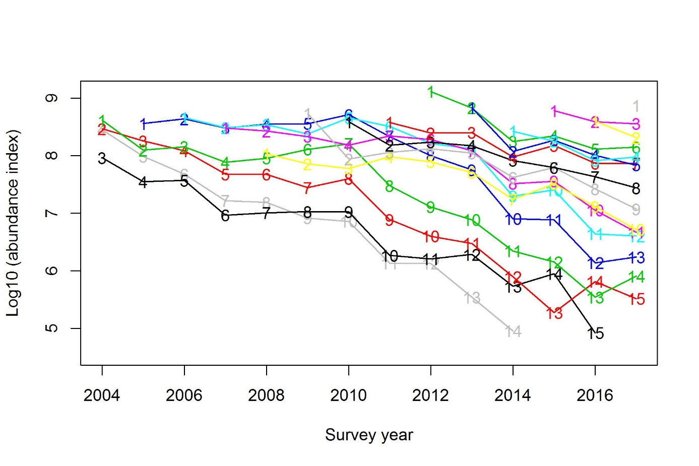
Figure 2. Log abundance of cod (individuals), swpet area estimates from the Barents Sea Ecosystem Survey. Each line represent a cohort, first cohort the 2000-cohort, last cohort 2016. The numbers correspond to age (1-15).
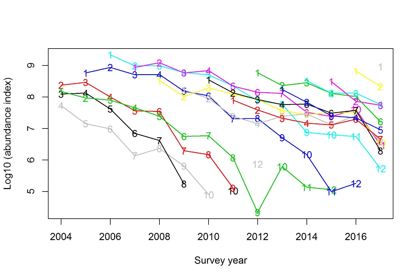
Figure 3. Log abundance haddock (individuals), swept area estimates from the Barents Sea Ecosystem Survey. Each line represent a cohort, first cohort the 2000-cohort, last cohort 2016. The numbers on the lines are the ages from 1 to 12. The dip at age 9 in 2012 might be caused by errors in age reading e.g. misreading haddock age 9 as haddock age 8 or 10. Age 9 in 2012 is from a weak cohort, and the uncertainty is high (see Table 7). Also note the upwards jump for many age classes in 2016, a year with lack of coverage in central/eastern Barents Sea.
3.1.2 - Mean length at age
Length at age of cod and haddock are given in Table 3 and 4, respectively.
Table 3. Mean length at age of cod (cm), data from bottom trawls Barents Sea Ecosystem survey.
| Year | 1 | 2 | 3 | 4 | 5 | 6 | 7 | 8 | 9 | 10 | 11 | 12 | 13 | 14 |
| 2004 | 14.5 | 24.1 | 36.2 | 45.2 | 55.2 | 66.0 | 73.1 | 81.0 | 89.9 | 100.9 | 124.6 | 119.0 | - | 117.8 |
| 2005 | 15.2 | 25.6 | 36.0 | 47.4 | 56.7 | 65.2 | 74.3 | 81.5 | 86.7 | 97.4 | 91.2 | - | 98.9 | - |
| 2006 | 16.6 | 25.8 | 36.8 | 49.2 | 58.5 | 67.7 | 75.1 | 82.6 | 90.5 | 102.6 | 98.3 | 96.0 | - | - |
| 2007 | 17.9 | 26.5 | 38.0 | 51.0 | 60.5 | 70.3 | 77.2 | 86.3 | 94.5 | 102.4 | - | 109.6 | - | 123.0 |
| 2008 | 16.1 | 27.8 | 38.5 | 49.9 | 59.7 | 70.3 | 77.9 | 86.0 | 93.0 | 98.9 | 105.3 | 104.4 | 123.0 | - |
| 2009 | 14.5 | 26.4 | 37.0 | 48.2 | 56.4 | 65.2 | 77.2 | 84.2 | 89.7 | 94.4 | 95.9 | 109.3 | 105.5 | - |
| 2010 | 15.3 | 25.8 | 38.0 | 47.3 | 56.5 | 66.0 | 74.3 | 83.5 | 90.9 | 94.9 | 99.0 | 100.3 | 112.8 | 116.8 |
| 2011 | 15.8 | 25.4 | 36.5 | 48.7 | 58.1 | 66.3 | 73.5 | 81.5 | 91.5 | 100.8 | 108.5 | 105.0 | 110.9 | - |
| 2012 | 15.3 | 25.4 | 36.0 | 46.2 | 57.2 | 65.1 | 72.5 | 79.3 | 90.1 | 97.8 | 103.8 | 107.3 | 114.9 | 108.0 |
| 2013 | 14.9 | 24.0 | 36.6 | 46.8 | 55.9 | 63.8 | 71.7 | 79.4 | 86.6 | 96.8 | 102.0 | 110.4 | 115.4 | 122.5 |
| 2014 | 14.3 | 25.3 | 35.1 | 47.2 | 57.6 | 64.5 | 75.6 | 82.0 | 88.9 | 94.6 | 96.1 | 108.8 | 93.5 | 114.0 |
| 2015 | 14.5 | 24.4 | 36.1 | 45.4 | 55.4 | 65.3 | 72.5 | 81.6 | 87.7 | 93.4 | 98.4 | 110.2 | 108.5 | 122.2 |
| 2016 | 16.7 | 26.0 | 38.1 | 47.1 | 56.1 | 64.6 | 73.2 | 80.9 | 90.6 | 94.7 | 98.3 | 106.3 | 98.1 | 118.1 |
| 2017 | 16.2 | 27.1 | 36.3 | 47.0 | 56.9 | 65.0 | 73.0 | 82.3 | 87.5 | 92.0 | 95.3 | 102.2 | 110.6 | 110.1 |
Table 4. Mean length at age of haddock (cm), data from bottom trawls Barents Sea Ecosystem survey.
| Year | 1 | 2 | 3 | 4 | 5 | 6 | 7 | 8 | 9 | 10 | 11 | 12 | 13 | 14 |
| 2004 | 18.5 | 25.4 | 32.7 | 41.6 | 47.7 | 51.6 | 56.8 | 63.6 | - | 68.0 | - | 72.6 | 71.5 | - |
| 2005 | 19.4 | 23.3 | 34.5 | 38.7 | 48.4 | 49.5 | 55.2 | 62.1 | 66.8 | 70.5 | 64.1 | 66.0 | - | - |
| 2006 | 20.8 | 28.0 | 35.4 | 41.6 | 46.3 | 52.8 | 54.8 | 56.3 | 67.2 | 68.5 | 71.1 | 69.0 | - | - |
| 2007 | 20.9 | 27.8 | 35.0 | 41.7 | 48.1 | 49.0 | 54.7 | 59.5 | 61.1 | 69.5 | 66.9 | 66.9 | - | - |
| 2008 | 20.4 | 28.5 | 34.2 | 40.5 | 46.8 | 49.8 | 57.3 | 55.8 | 62.0 | 62.9 | - | - | - | - |
| 2009 | 19.6 | 27.5 | 35.8 | 40.5 | 42.8 | 48.3 | 54.1 | 57.7 | 61.0 | 69.0 | - | - | - | - |
| 2010 | 18.6 | 24.0 | 34.2 | 40.6 | 45.2 | 50.3 | 52.9 | 59.0 | - | 70.0 | 70.0 | 58.0 | - | - |
| 2011 | 18.1 | 26.1 | 33.1 | 43.4 | 46.1 | 49.8 | 54.0 | 59.1 | 63.9 | 65.8 | - | 62.0 | 71.0 | - |
| 2012 | 19.4 | 25.5 | 36.0 | 36.2 | 47.8 | 49.7 | 52.3 | 54.2 | 65.0 | - | - | 70.6 | 68.5 | 86.0 |
| 2013 | 18.3 | 26.5 | 33.7 | 44.7 | 47.6 | 52.4 | 53.6 | 55.6 | 59.0 | 55.7 | - | - | 65.0 | - |
| 2014 | 19.3 | 24.3 | 36.3 | 43.4 | 49.6 | 54.2 | 55.9 | 56.9 | 58.6 | 63.4 | 70.0 | - | - | - |
| 2015 | 18.7 | 27.0 | 33.4 | 44.5 | 52.4 | 55.3 | 56.3 | 58.7 | 60.0 | 62.0 | 68.0 | 68.5 | - | - |
| 2016 | 19.9 | 26.3 | 37.2 | 42.2 | 51.8 | 54.1 | 58.7 | 60.0 | 62.1 | 62.2 | 67.9 | 72.0 | 79.0 | - |
| 2017 | 19.6 | 27.8 | 37.1 | 44.9 | 52.6 | 55.6 | 60.1 | 60.9 | 62.4 | 61.6 | 62.5 | 68.6 | - | - |
3.1.3 - Weight at age
Weight at age of cod and haddock are given in Table 5 and 6, respectively.
Table 5. Mean weight at age of cod (g), data from bottom trawls Barents Sea Ecosystem survey.
| Year | 1 | 2 | 3 | 4 | 5 | 6 | 7 | 8 | 9 | 10 | 11 | 12 | 13 | 14 |
| 2004 | 30 | 127 | 415 | 823 | 1464 | 2448 | 3266 | 4608 | 6323 | 9444 | 18331 | 13830 | - | 15924 |
| 2005 | 37 | 162 | 428 | 985 | 1723 | 2553 | 3697 | 4808 | 5958 | 8583 | 7662 | - | 8799 | - |
| 2006 | 39 | 155 | 473 | 1068 | 1759 | 2723 | 3725 | 5220 | 6798 | 10769 | 8904 | 9520 | - | - |
| 2007 | 52 | 173 | 523 | 1237 | 2078 | 3004 | 4163 | 5860 | 7638 | 11251 | - | 12683 | - | 15529 |
| 2008 | 39 | 193 | 511 | 1154 | 1958 | 3187 | 4262 | 5793 | 7741 | 9563 | 12039 | 11149 | 16320 | - |
| 2009 | 29 | 164 | 462 | 989 | 1614 | 2453 | 4034 | 5313 | 6334 | 7595 | 8221 | 12001 | 12040 | - |
| 2010 | 37 | 152 | 470 | 946 | 1634 | 2551 | 3801 | 5381 | 6921 | 7986 | 9063 | 8868 | 13406 | 19217 |
| 2011 | 35 | 143 | 419 | 991 | 1672 | 2523 | 3500 | 4812 | 6826 | 9403 | 12623 | 10379 | 10945 | - |
| 2012 | 34 | 149 | 418 | 904 | 1634 | 2388 | 3276 | 4344 | 6466 | 8459 | 9798 | 11181 | 14621 | 10895 |
| 2013 | 28 | 129 | 429 | 918 | 1553 | 2249 | 3230 | 4443 | 5805 | 8454 | 9817 | 12531 | 14308 | 17723 |
| 2014 | 28 | 148 | 374 | 897 | 1684 | 2244 | 3501 | 4511 | 5933 | 7183 | 7894 | 11979 | 7602 | 13250 |
| 2015 | 28 | 149 | 414 | 823 | 1483 | 2297 | 3219 | 4490 | 5635 | 6962 | 8478 | 12148 | 10385 | 15370 |
| 2016 | 45 | 162 | 527 | 914 | 1563 | 2308 | 3324 | 4492 | 6472 | 7476 | 8689 | 10939 | 7485 | 16645 |
| 2017 | 37 | 185 | 441 | 953 | 1660 | 2414 | 3398 | 4821 | 5876 | 7173 | 8345 | 9968 | 12765 | 12445 |
Table 6. Mean weight at age of haddock (g), data from bottom trawls Barents Sea Ecosystem survey.
| Year | 1 | 2 | 3 | 4 | 5 | 6 | 7 | 8 | 9 | 10 | 11 | 12 | 13 | 14 |
| 2004 | 59 | 168 | 348 | 697 | 1053 | 1355 | 1820 | 2621 | - | 3119 | - | 3950 | 3649 | - |
| 2005 | 75 | 146 | 436 | 654 | 1117 | 1218 | 1733 | 2283 | 2970 | 2989 | 2505 | 3184 | - | - |
| 2006 | 89 | 224 | 455 | 770 | 1011 | 1479 | 1685 | 1911 | 2937 | 3192 | 4185 | 2708 | - | - |
| 2007 | 96 | 227 | 441 | 896 | 1211 | 1214 | 1861 | 2095 | 2463 | 3296 | 3370 | 3490 | - | - |
| 2008 | 87 | 238 | 402 | 685 | 1082 | 1302 | 1866 | 1819 | 2482 | 2313 | - | - | - | - |
| 2009 | 76 | 221 | 445 | 667 | 842 | 1163 | 1509 | 2228 | 2276 | 3049 | - | - | - | - |
| 2010 | 66 | 149 | 384 | 632 | 921 | 1334 | 1524 | 2187 | - | 3254 | 2345 | 1970 | - | - |
| 2011 | 55 | 180 | 360 | 793 | 947 | 1242 | 1583 | 2084 | 2415 | 2340 | - | 2112 | 2632 | - |
| 2012 | 77 | 184 | 495 | 510 | 1120 | 1239 | 1445 | 1675 | 2552 | - | - | 3141 | 2929 | 4915 |
| 2013 | 60 | 183 | 397 | 912 | 1046 | 1404 | 1491 | 1685 | 2013 | 1950 | - | - | 2950 | - |
| 2014 | 68 | 169 | 494 | 859 | 1212 | 1549 | 1640 | 1721 | 1947 | 2299 | 3355 | - | - | - |
| 2015 | 67 | 218 | 416 | 913 | 1408 | 1649 | 1806 | 2003 | 2149 | 2250 | 2690 | 3030 | - | - |
| 2016 | 80 | 214 | 524 | 795 | 1406 | 1633 | 2023 | 2140 | 2363 | 2330 | 3055 | 3541 | 4300 | - |
| 2017 | 74 | 221 | 531 | 949 | 1444 | 1693 | 2118 | 2209 | 2508 | 2367 | 2398 | 2915 | - | - |
3.2 - Quality evaluation
3.2.1 - Coefficients of variation
Table 7. Cod. Estimates of coefficient of variation (CV) for swept area abundance - see Table 1.
| Year | 1 | 2 | 3 | 4 | 5 | 6 | 7 | 8 | 9 | 10 | 11 | 12 | 13 | 14 | 15 |
| 2004 | 0.26 | 0.16 | 0.18 | 0.31 | 0.30 | 0.15 | 0.16 | 0.14 | 0.20 | 0.31 | 0.65 | 0.96 | - | 0.59 | - |
| 2005 | 0.16 | 0.16 | 0.16 | 0.18 | 0.15 | 0.12 | 0.11 | 0.13 | 0.32 | 0.32 | 0.55 | - | 0.92 | - | - |
| 2006 | 0.10 | 0.14 | 0.14 | 0.18 | 0.17 | 0.13 | 0.12 | 0.14 | 0.17 | 0.37 | 0.51 | 0.85 | - | - | - |
| 2007 | 0.19 | 0.15 | 0.16 | 0.19 | 0.29 | 0.17 | 0.13 | 0.18 | 0.30 | 0.52 | - | 0.67 | - | 0.95 | - |
| 2008 | 0.17 | 0.15 | 0.14 | 0.21 | 0.17 | 0.18 | 0.18 | 0.15 | 0.20 | 0.27 | 0.51 | 0.92 | 0.99 | - | - |
| 2009 | 0.12 | 0.15 | 0.25 | 0.22 | 0.31 | 0.29 | 0.12 | 0.13 | 0.14 | 0.19 | 0.26 | 0.57 | 0.67 | - | - |
| 2010 | 0.10 | 0.15 | 0.18 | 0.18 | 0.25 | 0.39 | 0.35 | 0.35 | 0.33 | 0.33 | 0.42 | 0.65 | 0.52 | 0.76 | - |
| 2011 | 0.19 | 0.16 | 0.17 | 0.25 | 0.16 | 0.17 | 0.17 | 0.16 | 0.14 | 0.26 | 0.25 | 0.43 | 0.51 | - | - |
| 2012 | 0.11 | 0.17 | 0.15 | 0.18 | 0.24 | 0.22 | 0.13 | 0.18 | 0.14 | 0.14 | 0.28 | 0.26 | 0.41 | 0.61 | 0.71 |
| 2013 | 0.08 | 0.11 | 0.14 | 0.15 | 0.17 | 0.14 | 0.19 | 0.13 | 0.13 | 0.14 | 0.18 | 0.32 | 0.38 | 0.42 | 0.62 |
| 2014* | 0.12 | 0.14 | 0.18 | 0.15 | 0.19 | 0.19 | 0.17 | 0.19 | 0.13 | 0.13 | 0.25 | 0.32 | 0.41 | 0.92 | 0.82 |
| 2015 | 0.11 | 0.17 | 0.20 | 0.23 | 0.17 | 0.15 | 0.18 | 0.11 | 0.14 | 0.17 | 0.17 | 0.30 | 0.64 | 0.42 | - |
| 2016 | 0.19 | 0.27 | 0.25 | 0.25 | 0.14 | 0.14 | 0.12 | 0.13 | 0.17 | 0.16 | 0.17 | 0.28 | 0.53 | 0.49 | 1.06 |
| 2017 | 0.09 | 0.12 | 0.28 | 0.22 | 0.15 | 0.24 | 0.25 | 0.14 | 0.20 | 0.19 | 0.20 | 0.15 | 0.24 | 0.37 | 0.56 |
*not included in cod tuning
Table 7. Haddock Estimates of coefficient of variation (CV) for swept area abundance - see Table 1.
| Year | 1 | 2 | 3 | 4 | 5 | 6 | 7 | 8 | 9 | 10 | 11 | 12 |
| 2004 | 0.17 | 0.18 | 0.32 | 0.33 | 0.23 | 0.19 | 0.38 | 0.25 | - | 0.69 | - | 1.03 |
| 2005 | 0.16 | 0.19 | 0.44 | 0.63 | 0.32 | 0.38 | 0.30 | 0.39 | 0.36 | 0.73 | 0.69 | 0.60 |
| 2006 | 0.21 | 0.17 | 0.22 | 0.17 | 0.30 | 0.24 | 0.23 | 0.27 | 0.46 | 0.74 | 1.02 | 0.88 |
| 2007 | 0.14 | 0.20 | 0.50 | 0.58 | 0.28 | 0.31 | 0.52 | 0.27 | 0.89 | 0.43 | 0.88 | 0.87 |
| 2008 | 0.13 | 0.18 | 0.24 | 0.24 | 0.28 | 0.32 | 0.41 | 0.49 | 0.38 | 0.76 | - | - |
| 2009 | 0.21 | 0.17 | 0.26 | 0.33 | 0.27 | 0.31 | 0.42 | 0.66 | 0.56 | 0.96 | - | - |
| 2010 | 0.19 | 0.21 | 0.43 | 0.38 | 0.33 | 0.35 | 0.37 | 0.37 | - | 0.83 | 0.87 | 1.01 |
| 2011 | 0.23 | 0.50 | 0.24 | 0.51 | 0.26 | 0.34 | 0.27 | 0.43 | 0.82 | 1.00 | - | 0.90 |
| 2012 | 0.15 | 0.25 | 0.20 | 0.29 | 0.28 | 0.20 | 0.18 | 0.30 | 0.88 | - | - | 0.67 |
| 2013 | 0.23 | 0.19 | 0.30 | 0.34 | 0.42 | 0.25 | 0.20 | 0.24 | 0.39 | 0.82 | - | - |
| 2014 | 0.18 | 0.29 | 0.34 | 0.26 | 0.33 | 0.40 | 0.24 | 0.35 | 0.30 | 0.59 | 1.00 | - |
| 2015 | 0.16 | 0.27 | 0.32 | 0.30 | 0.24 | 0.22 | 0.46 | 0.24 | 0.25 | 0.42 | 0.86 | 1.09 |
| 2016 | 0.29 | 0.21 | 0.45 | 0.58 | 0.30 | 0.34 | 0.38 | 0.46 | 0.43 | 0.45 | 0.35 | 0.63 |
| 2017 | 0.15 | 0.19 | 0.23 | 0.27 | 0.26 | 0.23 | 0.43 | 0.33 | 0.33 | 0.34 | 0.34 | 0.43 |
3.2.2 - Consistency
The consistency was quantified as the correlation between the log abundance of each cohort at age a with the log abundances of the same cohort at older ages, and is presented here for cod ages 1 to 15 years (Figure 4 and 5), and haddock aged 1 to 12 (Figure 6).
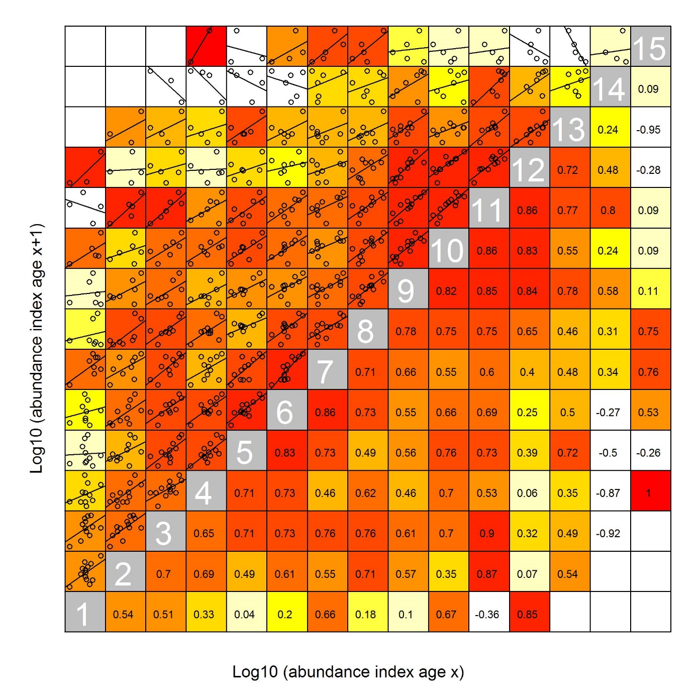
Figure 4. Cod internal consistency Barents Sea ecosystem survey 2004-2017, ages 1-15. The ages are shown in the grey squares on the diagonal. The numbers in the lower part of the matrix are the correlation coefficient between the log10 abundance of a cohort of age a with the log10 abundances of the same cohort at older ages. The upper part of the matrix plots the log10 abundance of a cohort of age a against the log10 abundances of the same cohort at older ages, plotted with the fitted regression line. Colours goes from deep red (high consistency, >0.8), to pale yellow (low consistency <0.1) and white, negative correlation.
In Figure 5, 2014 was removed from the cod data, since this year had poor coverage to the North (see Appendix Figure 11) Indices from BESS in 2018 is not included in the tuning series for the cod assessment (ICES 2019).
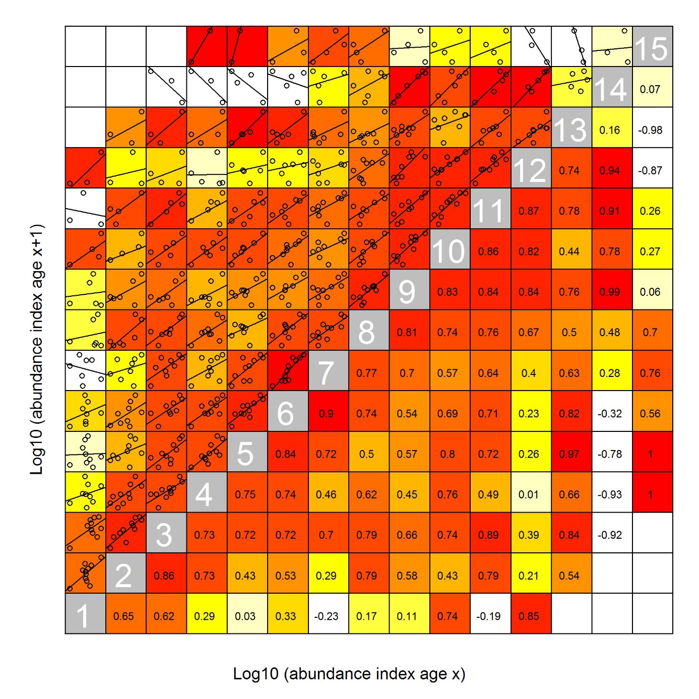
Figure 5. Cod internal consistency Barents Sea ecosystem survey 2004-2013 and 2015-2017, ages 1-15. The year 2014 was excluded due to lack of coverage in the northern Barents Sea (see appendix Figure 11) and is not used in the cod assessment. The ages are shown in the grey squares on the diagonal. The numbers in the lower part of the matrix are the correlation coefficient between the log10 abundance of a cohort of age a with the log10 abundances of the same cohort at older ages. The upper part of the matrix plots the log10 abundance of a cohort of age a against the log10 abundances of the same cohort at older ages, plotted with the fitted regression line. Colours goes from deep red (high consistency, >0.8), to pale yellow (low consistency <0.1) and white, negative correlations.
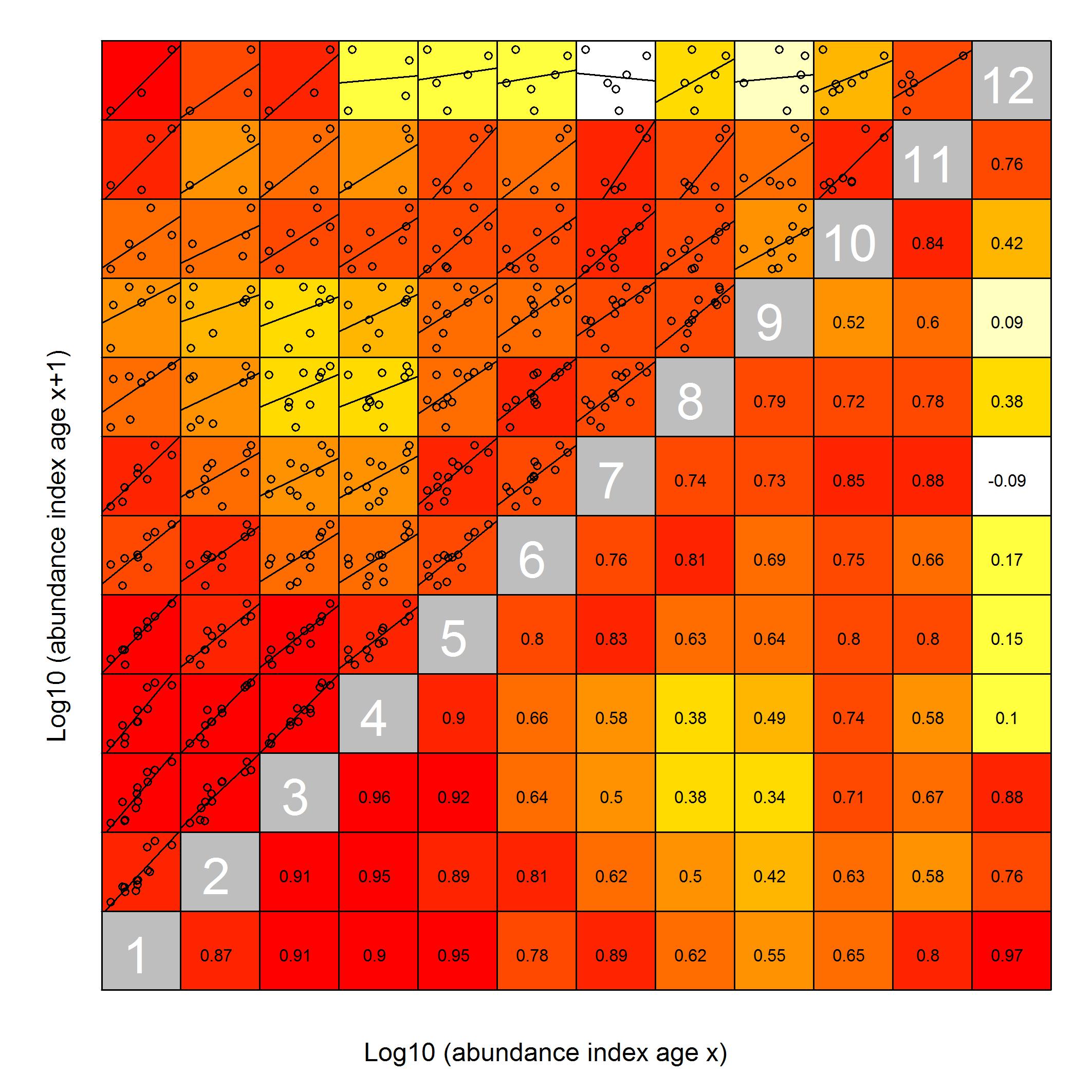
Figure 6. Haddock internal consistency Barents Sea ecosystem survey, 2004-2017, ages 1-15. The ages are shown in the grey squares on the diagonal. The numbers in the lower part of the matrix are the correlation coefficient between the log10 abundance of a cohort of age a with the log10 abundances of the same cohort at older ages. The upper part of the matrix plots the log10 abundance of a cohort of age a against the log10 abundances of the same cohort at older ages, plotted with the fitted regression line. Colours goes from deep red (high consistency, >0.8), to pale yellow (low consistency <0.1) and white, negative correlation.
4 - Conclusions and recommendations
The Barents Sea ecosystem survey (BESS) has many applications, one of the most important is the use of abundance indices from this survey in the annual cod and haddock assessments. A proper, comprehensive description and overview of the changes in survey design and sampling methods for BESS, similar to what has been provided for the winter survey by e.g. Jakobsen et al (1997) and Mehl et al (2016), has been lacking. We have here presented and compiled some of the relevant information on changes in design and sampling (see Appendix Table 1 and 2, Appendix Figures 1-15). Most notable, BESS has had incomplete spatial survey coverage due to ice hindrance in 2014, and due to technical problems and restricted access and trawl permits particularly in 2015, 2016 and 2018. In 2018 the coverage was too poor to be consider for index calculation for the cod and haddock assessments. We constructed a simplified strata system based on average densities of cod and haddock, that we modified by year to account for variation in sampling intensities. We used this strata system in StoX and Rstox to estimate abundance indices for cod and haddock and lengths and weights at age. We also quantified the uncertainty and consistencies of the survey indices.
Uncertainty measured as the coefficient of variation (CV) were much higher for haddock than for cod. This might be due to overall lower haddock abundance, a more restricted spatial distribution, and that haddock is patchier distributed. Higher CV for haddock than cod were also evident for the winter survey (Mehl et al 2016). Compared to the winter survey, that has a denser station grid, the BESS CVs for both species were higher, but this was clearly much more pronounced for haddock. Some years appeared to have higher uncertainties than others. Cod uncertainties for older ages were high in 2010, a few very high catches in the eastern Barents Sea is likely responsible for this. Also, CVs for all ages of haddock were >0.2 in 2016, a year with a large hole in coverage in the central/eastern Barents Sea. Despite high CVs for haddock, the internal consistency was quite good also for haddock and comparable to the consistencies for cod. The survey tracked the declines in cohorts over time, and the correlation between the log abundance of a cohort at age a in year y with the log abundances of the same cohort at age a +1 in year y +1, was ≥ 0.73 for both cod and haddock of ages used in tuning.
Abundance estimates from BESS used in the Arctic Fisheries Working Group (ICES 2019) for assessment tuning is provided by PINRO, Russia and estimated using the BIOFOX software (Prozorkevich and Gjøsæter 2014). The internal consistency is higher for the haddock abundances estimated using BIOFOX compared to StoX, whereas consistency is almost identical for cod (Johannesen et al 2019). BIOFOX included extra demersal stations set out at acoustic registrations some years (Russian vessels only) and BIOFOX uses spatial interpolation by depth and distance (Prozorkevich and Gjøsæter 2014). This method appears to partly adjust for holes in the survey coverage and the large distance between the stations relatively to the patchy distribution of haddock.
We recommend that the BESS survey design should be kept constant from year to year, to make inter-annual variation in distributions etc easier to detect. If changes are to be made to the design, sampling gear etc, we recommended that the changes are based on relevant data analyses and biological knowledge and that they are well documented. BESS is a cooperation between Russia and Norway. Any change in the survey design and sampling must be agreed by both parties. Sampling methods are harmonized between the two countries, still there are issues related to e.g. sampling gear (Appendix Table 2), frequency (and use) of stations at dense acoustic registrations and data exchange and conversion that should be improved. A denser station grid in the main distribution area of haddock would probably improve the indices for this species and should be considered. More sophisticated methods for index calculations than presented here, e.g. geostatistical methods/delta-gam methods taking e.g. depth or other habitat characteristics into account, could perhaps amend some of the issues related to area and year variation in sampling intensities, large interstation distance and holes in the coverage, and should be considered. However, incomplete survey coverage (reduced extent and holes) will always increase uncertainty, there are no straightforward way to account for it, and it should therefore be avoided.
5 - References
ICES (2019). Arctic Fisheries Working Group (AFWG). ICES Scientific Reports. 1:30. 930 pp.
Jakobsen T, Korsbrekke K, Mehl S and Nakken O (1997). Norwegian combined acoustic and bottom trawl surveys for demersal fish in the Barents Sea during winter. ICES CM Y: 17.
Johannesen E, Johansen GO and Prozorkevich D (2019). WD_03. Cod and haddock abundance indices by age from the ecosystem survey: comparing current indices from BIOFOX and new indices from StoX. AFWG 2019.
Johnsen E , Totland A , Skålevik Å , et al. (2019). StoX: An open source software for marine survey analyses . Methods in Ecology and Evolution 2019 ; 10 : 1523 – 1528 . https://doi.org/10.1111/2041-210X.13250
Lepesevich YM and Shevelev M.S. (1997). Evolution of the Russian survey for demersal fish: from ideal to reality. ICES CM Y: 09.
Mehl S, Aglen A and Johnsen E (2016). Re-estimation of swept area indices with CVs for main demersal fish species in the Barents Sea winter survey 1994 – 2016 applying the Sea2Data StoX software. Fisken og Havet 10 2016.
Pavlenko A, Likhoshapko A, Prozorkevich D, Prokhorova T, Engås A, Aasen A and Eriksen E (2014). Report from the meeting between experts from PINRO and IMR to discuss sampling trawl methodology. Murmansk 28-29. January 2014. Unpublished report. 4 pp.
Prozorkevich D and Gjøsæter H (2014). WD_02 cod_BESS_assessment. AFWG 2014.
6 - Appendix Table 1 Overview of the data
Appendix table 1. Year: survey year; NO : name of participating Norwegian vessels; RU: Russian vessels; Days: the total number of survey days in that year – nb taken partly from survey reports and partly from data and therefore not 100% accurate; Stations: the number of all valid bottom trawl hauls, includes also hauls taken outside the strata system, see Appendix figures 1-15, Measured: total number of aged/length measured/ weighed individuals
| Year | NO | RU | Days | Stations | Measured |
| 2004 | Johan Hjort | F. Nansen | 230 | 600 | |
| Jan Mayen* | Smolensk | Haddock: 745/9960/746 | |||
| Cod: 2674/24005/2680 | |||||
| 2005 | GO Sars | F. Nansen | 228 | 625 | |
| Johan Hjort | Smolensk | Haddock: 955/10639/965 | |||
| Jan Mayen | Cod: 2267/14890/2594 | ||||
| 2006 | GO Sars | F. Nansen | 204 | 638 | |
| Johan Hjort | Smolensk | Haddock: 1174/29469/1252 | |||
| Jan Mayen | Cod: 2947/25856/3036 | ||||
| 2007 | GO Sars | Vilnius | 206 | 498 | |
| Johan Hjort | Smolensk | Haddock: 719/14096/788 | |||
| Jan Mayen | Cod: 1507/11727/1594 | ||||
| 2008** | GO Sars | Vilnius | 131 | 387 | |
| Johan Hjort | Haddock: 964/14036/967 | ||||
| Jan Mayen | Cod: 2464/15168/2473 | ||||
| 2009 | GO Sars | Vilnius | 127 | 357 | |
| Johan Hjort | Haddock: 1453/18581/1550 | ||||
| Jan Mayen | Cod: 2761/13922/2868 | ||||
| 2010 | GO Sars | Vilnius | 127 | 322 | |
| Johan Hjort | F. Nansen | Haddock: 1035/9743/1032 | |||
| Jan Mayen | Cod: 3099/15675/3089 | ||||
| 2011 | Christina E*** | Vilnius | 123 | 379 | |
| Johan Hjort | Haddock: 675/5512/681 | ||||
| Jan Mayen | Cod: 2397/18538/2443 | ||||
| 2012 | GO Sars | Vilnius | 152 | 428 | |
| Johan Hjort | Haddock: 902/9158/912 | ||||
| Helmer Hanssen | Cod: 3083/28066/3268 | ||||
| 2013 | GO Sars | Vilnius**** | 172 | 416 | |
| Johan Hjort | Haddock: 1103/7876/1109 | ||||
| Helmer Hanssen | Cod: 3957/28944/3965 |
| 2014 | GO Sars | Vilnius | 138 | 294 | |
| Johan Hjort | Haddock: 666/6680/672 | ||||
| Helmer Hanssen | Cod: 1782/11348/1808 | ||||
| 2015 | GO Sars | Vilnius | 140 | 326 | |
| Johan Hjort | Haddock: 742/6377/772 | ||||
| Helmer Hanssen | Cod: 2279/12163/2314 | ||||
| 2016 | Eros*** | F. Nansen | 139 | 294 | |
| Johan Hjort | Haddock: 800/6527/809 | ||||
| Helmer Hanssen | Cod: 2311/11214/2341 | ||||
| 2017 | GO Sars | Vilnius | 142 | 327 | |
| Johan Hjort | Haddock: 705/8171/787 | ||||
| Helmer Hanssen | Cod: 2395/15817/2408 | ||||
| 2018 | GO Sars | Vilnius | 138 | 214 | |
| Johan Hjort | |||||
| Helmer Hanssen |
*Jan Mayen renamed Helmer Hanssen in 2012
**Commercial vessel Atlantic Star took some pelagic hauls as part of the survey
***Commercial vessel Christina E and Eros replaced GO Sars in 2011 and 2016
****Access restricted to part of the REZ for Vilnius, so survey was extended one month for this vessel
7 - Appendix Table 2 Details on trawling procedures
Table 2 a. Overview of rigging and trawling procedure for the Campelen 1800 trawl used by IMR and PINRO, from Pavlenko et al (2014).
| Parameters | Russian | Norwegian | comments | *Significant differences |
| Trawl doors | 4.5 m2 (1250 kg), 5m2 (1460 kg), 6,5 m2 (1650 kg), universal (bottom/pelagic) | Jhjort and H.Hanssen-125 inch, Thyborøn, Type 7, 7.81m2, 1670kg; GOSars- 120 inch, Thyboroen, Type 12A, 7.93m2, 1861kg | Russian trawl doors change due to availability | * |
| Distance betwwen doors | 47-53m | 50±2m | Norway use constraining rope | |
| Warp/depth ratio | 2.5-4.5 depends on depths | 2.5-4.5 depends on depths | ||
| Bridle length | 40m | 40m | ||
| Rigging of ground gear | rockhopper's diameter- 35cm, tickler chain infront of rockhopper (4-5m); bobbins 8 m infront of ground gear | rockhopper's diameter- 35cm | tickler chain used only for ecosystem survey | * |
| Floats on headline | 90 floats of 2.8 buoyancy kg each | 90 floats of 2.8 buoyancy kg each | ||
| Floats on fishing line | no floats, 20-25 cm ropes between fishing line and upper chain of rockhopper | Tromsø rigging: 45 floats on fishing line and 18 floats of 8 inch in the extension. 10 cm ropes between fishing line and upper chain of rockhopper | * | |
| Monitoring gear perfomance | Wesmar sonar used only some times during the survey to check trawl performance | Acoustic trawl sensors (door spread, speed and vertical opening) | Russian vessels need to use permanently monitoring gear performance | * |
| Trawl design | equal | equal | ||
| Trawl opening | 15m horizontal and 4 m vertical | 4m vertical opening | ||
| Trawling procedure | Trawling duration 15 min after bottom contact | Trawling duration 15 min after bottom contact | ||
| Speed | 3-3.2 kn (GPS) | 3 kn( through water) |
Table 2 b. Overview of rigging and trawling procedure for the Campelen 1800 trawl used by IMR and PINRO, from the March meeting protocol 2019.
| Parameters | Russian vessels | Norwegian vessels | Comments | Significant differences between PINRO and IMR | Significant differences from 2014 |
| Trawl doors | Sparrow(1650 kg) | Thyborøn 7a(1800 kg)- all vessels | * | *IMR *PINRO | |
| Distance between doors | 47-55 m | 50±2 m | PINRO and IMR use constraining rope | *PINRO | |
| Warp/depth ratio | 2.0- 4.5. Depends on depth.Depends on trawl master/cruise leader | 2.5-4.5. Depends on depth. Norwegian vessels use information from roll sensors-trawl doors | * | ||
| Bridle length | 40m | 40m | |||
| Rigging of ground gear | Using 20 -25 cm rope between fishing line and ground gear | Rockhopper’s -diameter 35 cm | PINRO rigging, reason to expect that center fishing line behind and close to seabed- resulting in higher catch rates of benthos etc. compared to Norwegian rigging | PINRO has not used tickler chain from 2015 | *PINRO |
| Floats on headline | Total buoyancy 236 kg | Total buoyancy 261 kg±2 kg | |||
| Floats on fishing line and extension | Norwegian vessels, Tromsø rigging (used on some few stations in the Svalbard area, soft bottom): Floats on fishing line (bouncy 130kg±2 kg) and on the extension (bouncy 52 kg±2 kg) | * | *IMR | ||
| Monitoring gear performance | Acoustic trawl sensors: door spread, roll and pitch of doors, speed, vertical opening | Acoustic trawl sensors: door spread, roll and pitch of doors, speed, vertical opening | *PINRO | ||
| Trawl design | Equal | Equal | |||
| Trawl opening | Approx. 4 m | 3.8-4.2 m | |||
| Trawling procedure | Trawling duration 15 min after bottom contact | Trawling duration 15 min after bottom contact | |||
| Speed | 3 kn (speed over ground, GPS) | 3 kn (through water) | * |
8 - Appendix Figures 1-15 Maps of stations and strata by year
Appendix Figure 1. 2004. Stations grid set out according to 0-group survey design with Mercator projection. Approximately 35 nautical mile grid station distance. Denser grid was due to Greenland halibut juvenile investigation in Storfjordrenna, and west and east of Svalbard, and due to this the “Great Bank” stratum is split to account for the denser sampling in the western part of this stratum. The extent of the “ South East” stratum is reduced due to limited sampling coverage .
Appendix Figure 2. 2005. Stations set out in a modified UTM with approximately 35 nautical mile grid station distance. Denser grid was due to Greenland halibut juvenile investigation in Storfjordrenna, and west and east of Svalbard, and shrimp investigations in the Bear Island trough. Due to this, the “Great Bank” stratum is split to account for the denser sampling in the western part of this stratum, and the eastern part of this stratum is added to the “North East” stratum to obtain sufficient sample size. The “South West” stratum was split in two for the same reasons. Northern and eastern edges was reduced due to limited sampling coverage.
 Appendix Figure 3. 2006. Stations set out in a modified UTM with approximately 35 nautical mile grid station distance. Denser grid was due to Greenland halibut juvenile investigation in Storfjordrenna, and west and east of Svalbard and shrimp investigations in the Bear Island trough. The “Great Bank”, “Bear Island Through”, “South East” (flatfish investigations) and “South West strata were modified to account for denser sampling. Northern and eastern edges was reduced due to limited sampling coverage.
Appendix Figure 4. 2007. Stations set out in a modified UTM with approximately 35 nautical mile grid station distance. Denser grid was due to Greenland halibut juvenile investigation in Storfjordrenna, and west and east of Svalbard, and shrimp investigations in the Bear Island trough. The “Great Bank” stratum was split to account for denser sampling. North-eastern and eastern edges was reduced due to limited sampling coverage.
Appendix Figure 5. 2008. Stations set out in a modified UTM with approximately 35 nautical mile grid station distance. Denser grid was due to Greenland halibut juvenile investigation in Storfjordrenna, and west and east of Svalbard and shrimp investigations in the Bear Island trough. The sampling effort was regarded as fairly regular compared to earlier years, so the only modification was reduction of the northern edges due to limited survey coverage. This year suffered a strong reduction in Norwegian survey time due to budget cuts.
Appendix Figure 6. 2009. Stations set out in a modified UTM with approximately 35 nautical mile grid station distance. Denser grid west of Svalbard due to steep depth gradients. Reduction of the northern edges due to limited survey coverage. Russian investigations in Kara Sea (North east) not included in StoX calculations.
Appendix Figure 7. 2010. Stations set out in a modified UTM with approximately 35 nautical mile grid station distance. Reduction of the northern edges due to limited survey coverage. Russian investigations in Kara Sea (North east) not included in StoX calculations.
Appendix Figure 8. 2011. Stations set out in a modified UTM with approximately 35 nautical mile grid station distance. Denser grid west of Svalbard due to steep depth gradients. Reduction of the northern edges due to limited survey coverage. Russian investigations in Kara Sea (North east) not included in StoX calculations.
Appendix Figure 9. 2012. Stations set out in a modified UTM with approximately 35 nautical mile grid station distance, except around Svalbard. Denser grid west of Svalbard due to steep depth gradients. Reduction of the north-eastern edges due to limited survey coverage. Russian investigations in Kara Sea (North east) not included in StoX calculations.
Appendix Figure 10. 2013. Stations set out in a modified UTM with approximately 35 nautical mile grid station distance, except around Svalbard. Denser grid west of Svalbard due to steep depth gradients. Reduction of the north-eastern edges due to limited survey coverage.
Appendix Figure 11. 2014. Stations set out in a modified UTM with approximately 35 nautical mile grid station distance, except around Svalbard. Denser grid west of Svalbard due to steep depth gradients. Reduction of the northern edges due to limited survey coverage. NB! Ice restrictions in the north – this year the survey indices were not used in the cod assessment.
Appendix Figure 12. 2015 Stations set out in a modified UTM with approximately 35 nautical mile grid station distance, except around Svalbard. Denser grid west of Svalbard due to steep depth gradients. No coverage in the loop hole due to unclear jurisdictions. Reduction of the northern edges due to limited survey coverage.
Appendix Figure 13. 2016. Stations set out in a modified UTM with approximately 35 nautical mile grid station distance, except around Svalbard. Denser grid west of Svalbard due to steep depth gradients. No coverage in loop hole due to unclear jurisdictions. Russian military exercise limited survey access to the south eastern BS. Reduction of the north-eastern edges due to limited survey coverage.
Appendix Figure 14. 2017. Stations set out with approximately 35 nautical mile grid station distance, according to Albers equal-area projection (also called: Albers Equal-Area Conic Projection) with the following parameter settings: Centre latitude: 75 N, Centre longitude: 30 E, 1st standard Latitude: 70 N, 2nd standard latitude: 80 N. Modified station grid in the western part to avoid deeper stations than 500 m, and around Svalbard due to restrictions in natural reserves. Some additional stations in “Spitsbergen Bank”, “Svalbard” and “Great Bank” strata to cover Greenland halibut. Slight reduction of the north-eastern and south-eastern edges due to limited survey coverage.
Appendix Figure 15. 2018. Stations set out with approximately 35 nautical mile grid station distance, according to Albers equal-area projection (also called: Albers Equal-Area Conic Projection) with the following parameter settings: Centre latitude: 75 N, Centre longitude: 30 E, 1st standard Latitude: 70 N, 2nd standard latitude: 80 N. Modified grid in the western part to avoid deeper stations than 500 m, and around Svalbard due to restrictions in natural reserves. Some additional stations in “Spitsbergen Bank”, “Svalbard” and “Great Bank” strata to cover Greenland halibut. Slight reduction of the north-eastern edges due to limited survey coverage. Lack of coverage in east was due technical problems with the Russian vessel. No attempt was done to calculate survey indices in 2018, due to this severe coverage problem.